which reads as follows: Ld is a set of functions, where each function is parameterized by w∈Rd and b∈R, and each such function takes as input a vector x and returns as output the scalar ⟨w,x⟩+b.
It may be more convenient to incorporate b, called the bias, into w as an extra coordinate and add an extra coordinate with a value of 1 to all x∈X; namely, let w′=(b,w1,w2,…wd)∈Rd+1 and let x′=(1,x1,x2,…,xd)∈Rd+1. Therefore
The first hypothesis class we consider is the class of halfspaces, designed for binary classification problems, namely, X=Rd and Y={−1,+1}. The class of halfspaces is defined as follows:
HSd=sign∘Ld={x↦sign(hw,b(x)):hw,b∈Ld}.
In other words, each halfspace hypothesis in HSd is parameterized by w∈Rd and b∈R and upon receiving a vector x the hypothesis returns the label sign(⟨w,x⟩+b)
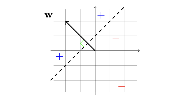
To illustrate this hypothesis class geometrically, it is instructive to consider the case d=2. Each hypothesis forms a hyperplane that is perpendicular to the vector w and intersects the vertical axis at the point (0,−b/w2). The instances that are "above" the hyperplane, that is, share an acute angle with w, are labeled positively. Instances that are "below" the hyperplane, that is, share an obtuse angle with w, are labeled negatively.
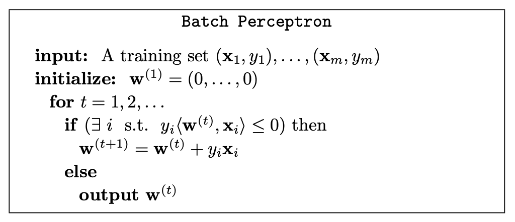
A different implementation of the ERM rule is the Perceptron algorithm of Rosenblatt (Rosenblatt 1958). The Perceptron is an iterative algorithm that constructs a sequence of vectors w(1),w(2),…. Initially, w(1) is set to be the all-zeros vector. At iteration t, the Perceptron finds an example i that is mislabeled by w(t), namely, an example for which sign(⟨w(t),xi⟩)=yi. Then, the Perceptron updates w(t) by adding to it the instance xi scaled by the label yi. That is, w(t+1)=w(t)+yixi. Recall that our goal is to have yi⟨w,xi⟩>0 for all i and note that
The Perceptron Learning Algorithm makes at most γ2R2 updates (after which it returns a separating hyperplane), where R is the largest norm of Xj′ 's and γ=minYj⟨w∗,Xj⟩ where ∥w∗∥2=1.
It is immediate from the code that should the algorithm terminate and return a weight vector, then the weight vector must separate the + points from the − points. Thus, it suffices to show that the algorithm terminates after at most γ2R2 updates. In other words, we need to show that k is upper-bounded by γ2R2. Our strategy to do so is to derive both lower and upper and bounds on the length of wk+1 in terms of k, and to relate them.
Note that w1=0, and for k⩾1, note that if xj is the misclasssified point during iteration k, we have
wk+1⋅w⋆=(wk+yjxj)⋅w⋆=wk⋅w⋆+yj(xj⋅w⋆)>wk⋅w⋆+γ
It follows by induction that wk+1⋅w⋆>kγ. Since wk+1⋅w⋆⩽∥∥wk+1∥∥∥w⋆∥=∥∥wk+1∥∥, we get
The hypothesis class of linear regression predictors is simply the set of linear functions,
Hreg=Ld={x↦⟨w,x⟩+b:w∈Rd,b∈R}
Next we need to define a loss function for regression. While in classification the definition of the loss is straightforward, as ℓ(h,(x,y)) simply indicates whether h(x) correctly predicts y or not, in regression, if the baby's weight is 3kg, both the predictions 3.00001kg and 4kg are "wrong," but we would clearly prefer the former over the latter. We therefore need to define how much we shall be "penalized" for the discrepancy between h(x) and y. One common way is to use the squared-loss function, namely,
ℓ(h,(x,y))=(h(x)−y)2.
For this loss function, the empirical risk function is called the Mean Squared Error, namely,
Least squares is the algorithm that solves the ERM problem for the hypothesis class of linear regression predictors with respect to the squared loss. The ERM problem with respect to this class, given a training set S, and using the homogenous version of Ld, is to find
wargminLS(hw)=wargminm1i=1∑m(⟨w,xi⟩−yi)2.
To solve the problem we calculate the gradient of the objective function and compare it to zero. That is, we need to solve
m2i=1∑m(⟨w,xi⟩−yi)xi=0.
We can rewrite the problem as the problem Aw=b where
If A is invertible then the solution to the ERM problem is
w=A−1b.
The case in which A is not invertible requires a few standard tools from linear algebra. It can be easily shown that if the training instances do not span the entire space of Rd then A is not invertible. Nevertheless, we can always find a solution to the system Aw=b because b is in the range of A. Indeed, since A is symmetric we can write it using its eigenvalue decomposition as A=VDV⊤, where D is a diagonal matrix and V is an orthonormal matrix (that is, V⊤V is the identity d×d matrix). Define D+to be the diagonal matrix such that Di,i+=0 if Di,i=0 and otherwise Di,i+=1/Di,i. Now, define
A+=VD+V⊤ and w^=A+b.
Let vi denote the i 'th column of V. Then, we have
Aw^=AA+b=VDV⊤VD+V⊤b=VDD+V⊤b=i:Di,i=0∑vivi⊤b.
That is, Aw^ is the projection of b onto the span of those vectors vi for which Di,i=0. Since the linear span of x1,…,xm is the same as the linear span of those vi, and b is in the linear span of the xi, we obtain that Aw^=b, which concludes our argument.
Linear Regression for Polynomial Regression Tasks
Some learning tasks call for nonlinear predictors, such as polynomial predictors. Take, for instance, a one dimensional polynomial function of degree n, that is,
p(x)=a0+a1x+a2x2+⋯+anxn
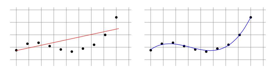
where (a0,…,an) is a vector of coefficients of size n+1. In the following we depict a training set that is better fitted using a 3rd degree polynomial predictor than using a linear predictor.
We will focus here on the class of one dimensional, n-degree, polynomial regression predictors, namely,
Hpoly n={x↦p(x)},
where p is a one dimensional polynomial of degree n, parameterized by a vector of coefficients (a0,…,an). Note that X=R, since this is a one dimensional polynomial, and Y=R, as this is a regression problem.
One way to learn this class is by reduction to the problem of linear regression, which we have already shown how to solve. To translate a polynomial regression problem to a linear regression problem, we define the mapping ψ:R→Rn+1 such that ψ(x)=(1,x,x2,…,xn). Then we have that
p(ψ(x))=a0+a1x+a2x2+⋯+anxn=⟨a,ψ(x)⟩
and we can find the optimal vector of coefficients a by using the Least Squares algorithm as shown earlier.
In logistic regression we learn a family of functions h from Rd to the interval [0,1]. However, logistic regression is used for classification tasks: We can interpret h(x) as the probability that the label of x is 1 . The hypothesis class associated with logistic regression is the composition of a sigmoid function ϕsig :R→[0,1] over the class of linear functions Ld. In particular, the sigmoid function used in logistic regression is the logistic function, defined as
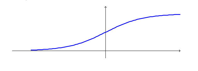
ϕsig (z)=1+exp(−z)1.
The name "sigmoid" means "S-shaped," referring to the plot of this function, shown in the figure:
The hypothesis class is therefore (where for simplicity we are using homogenous linear functions):
Hsig =ϕsig ∘Ld={x↦ϕsig (⟨w,x⟩):w∈Rd}.
Note that when ⟨w,x⟩ is very large then ϕsig (⟨w,x⟩) is close to 1 , whereas if ⟨w,x⟩ is very small then ϕsig (⟨w,x⟩) is close to 0 . Recall that the prediction of the halfspace corresponding to a vector w is sign(⟨w,x⟩). Therefore, the predictions of the halfspace hypothesis and the logistic hypothesis are very similar whenever ∣⟨w,x⟩∣ is large. However, when ∣⟨w,x⟩∣ is close to 0 we have that ϕsig (⟨w,x⟩)≈21. Intuitively, the logistic hypothesis is not sure about the value of the label so it guesses that the label is sign(⟨w,x⟩) with probability slightly larger than 50%. In contrast, the halfspace hypothesis always outputs a deterministic prediction of either 1 or −1, even if ∣⟨w,x⟩∣ is very close to 0 .
Next, we need to specify a loss function. That is, we should define how bad it is to predict some hw(x)∈[0,1] given that the true label is y∈{±1}. Clearly, we would like that hw(x) would be large if y=1 and that 1−hw(x) (i.e., the probability of predicting −1 ) would be large if y=−1. Note that
Therefore, any reasonable loss function would increase monotonically with 1+exp(y⟨w,x⟩)1, or equivalently, would increase monotonically with 1+exp(−y⟨w,x⟩). The logistic loss function used in logistic regression penalizes hw based on the log of 1+exp(−y⟨w,x⟩) (recall that log is a monotonic function). That is,
ℓ(hw,(x,y))=log(1+exp(−y⟨w,x⟩)).
Therefore, given a training set S=(x1,y1),…,(xm,ym), the ERM problem associated with logistic regression is
w∈Rdargminm1i=1∑mlog(1+exp(−yi⟨w,xi⟩)).
The advantage of the logistic loss function is that it is a convex function with respect to w; hence the ERM problem can be solved efficiently using standard methods. We will study how to learn with convex functions, and in particular specify a simple algorithm for minimizing convex functions, in later chapters.
The ERM problem associated with logistic regression is identical to the problem of finding a Maximum Likelihood Estimator, a well-known statistical approach for finding the parameters that maximize the joint probability of a given data set assuming a specific parametric probability function. We will study the Maximum Likelihood approach in Chapter 24.