Nonlinear Constrained Optimization - Equality

Problems with Equality Constraints

The class of optimization problems we analyze here is

$$\begin{aligned} \operatorname{minimize} & f(\boldsymbol{x}) \\ \text { subject to } & \boldsymbol{h}(\boldsymbol{x})=\mathbf{0} \end{aligned}$$

where $\boldsymbol{x} \in \mathbb{R}^{n}, f: \mathbb{R}^{n} \rightarrow \mathbb{R}, \boldsymbol{h}: \mathbb{R}^{n} \rightarrow \mathbb{R}^{m}, \boldsymbol{h}=\left[h_{1}, \ldots, h_{m}\right]^{\top}$, and $m \leq n$. We assume that the function $\boldsymbol{h}$ is continuously differentiable, that is, $\boldsymbol{h} \in \mathcal{C}^{1}$.

Definition

A point $x^{*}$ satisfying the constraints $h_{1}\left(x^{*}\right)=$ $0, \ldots, h_{m}\left(\boldsymbol{x}^{*}\right)=0$ is said to be a regular point of the constraints if the gradient vectors $\nabla h_{1}\left(\boldsymbol{x}^{*}\right), \ldots, \nabla h_{m}\left(\boldsymbol{x}^{*}\right)$ are linearly independent.

Let $\boldsymbol{D} \boldsymbol{h}\left(\boldsymbol{x}^{*}\right)$ be the Jacobian matrix of $\boldsymbol{h}=\left[h_{1}, \ldots, h_{m}\right]^{\top}$ at $\boldsymbol{x}^{*}$, given by

$$D \boldsymbol{h}\left(\boldsymbol{x}^{*}\right)=\left[\begin{array}{c} D h_{1}\left(\boldsymbol{x}^{*}\right) \\ \vdots \\ D h_{m}\left(\boldsymbol{x}^{*}\right) \end{array}\right]=\left[\begin{array}{c} \nabla h_{1}\left(\boldsymbol{x}^{*}\right)^{\top} \\ \vdots \\ \nabla h_{m}\left(\boldsymbol{x}^{*}\right)^{\top} \end{array}\right] .$$

Then, $\boldsymbol{x}^{*}$ is regular if and only if rank $D h\left(\boldsymbol{x}^{*}\right)=m$ (i.e., the Jacobian matrix is of full rank).

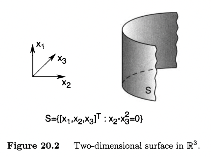
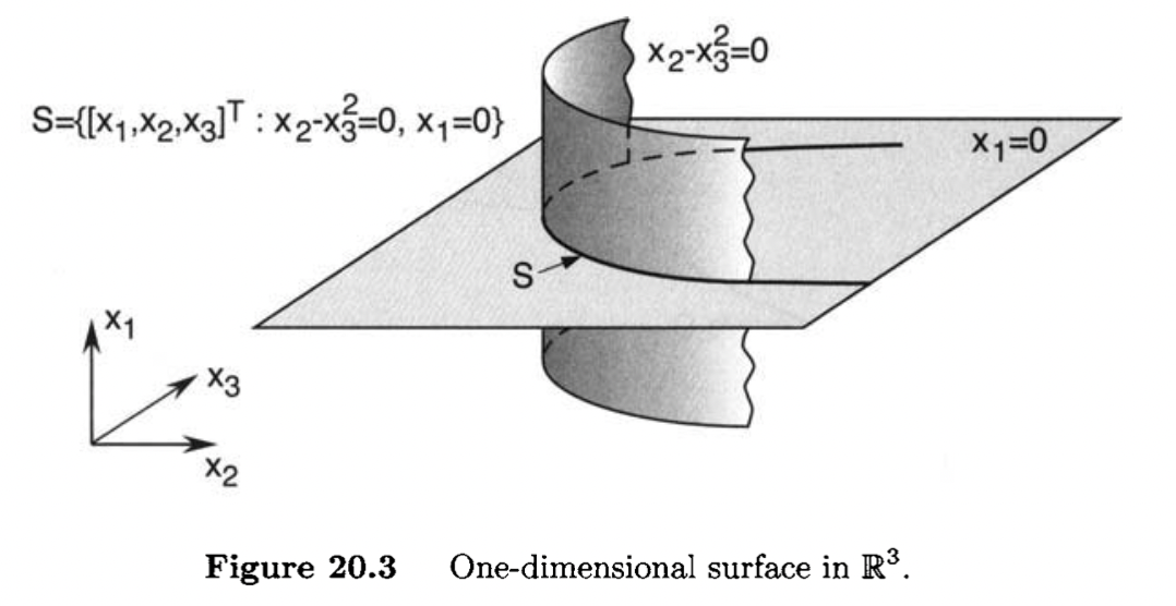
The set of equality constraints $h_{1}(\boldsymbol{x})=0, \ldots, h_{m}(\boldsymbol{x})=0, h_{i}: \mathbb{R}^{n} \rightarrow \mathbb{R}$, describes a surface

$$S=\left\{\boldsymbol{x} \in \mathbb{R}^{n}: h_{1}(\boldsymbol{x})=0, \ldots, h_{m}(\boldsymbol{x})=0\right\}$$

Assuming that the points in $S$ are regular, the dimension of the surface $S$ is $n-m$

Tangent and Normal Spaces

In this section we discuss the notion of a tangent space and normal space at a point on a surface. We begin by defining a curve on a surface $S$.

Definition

A curve $C$ on a surface $S$ is a set of points $\{\boldsymbol{x}(t) \in S: t \in$ $(a, b)\}$, continuously parameterized by $t \in(a, b) ;$ that is, $\boldsymbol{x}:(a, b) \rightarrow S$ is a continuous function.

A graphical illustration of the definition of a curve is given in Figure 20.4. The definition of a curve implies that all the points on the curve satisfy the equation describing the surface. The curve $C$ passes through a point $\boldsymbol{x}^{*}$ if there exists $t^{*} \in(a, b)$ such that $\boldsymbol{x}\left(t^{*}\right)=\boldsymbol{x}^{*}$.

Intuitively, we can think of a curve $C=\{x(t): t \in(a, b)\}$ as the path traversed by a point $\boldsymbol{x}$ traveling on the surface $S$. The position of the point at time $t$ is given by $\boldsymbol{x}(t)$.

Definition

The curve $C=\{\boldsymbol{x}(t): t \in(a, b)\}$ is differentiable if

$$\dot{\boldsymbol{x}}(t)=\frac{d \boldsymbol{x}}{d t}(t)=\left[\begin{array}{c} \dot{x}_{1}(t) \\ \vdots \\ \dot{x}_{n}(t) \end{array}\right]$$

exists for all $t \in(a, b)$.

Figure 20.4 Curve on a surface.

Figure 20.5 Geometric interpretation of the differentiability of a curve.

The curve $C=\{\boldsymbol{x}(t): t \in(a, b)\}$ is twice differentiable if

$$\ddot{\boldsymbol{x}}(t)=\frac{d^{2} \boldsymbol{x}}{d t^{2}}(t)=\left[\begin{array}{c} \ddot{x}_{1}(t) \\ \vdots \\ \ddot{x}_{n}(t) \end{array}\right]$$

exists for all $t \in(a, b)$.

Note that both $\dot{x}(t)$ and $\ddot{x}(t)$ are $n$-dimensional vectors. We can think of $\dot{\boldsymbol{x}}(t)$ and $\ddot{\boldsymbol{x}}(t)$ as the velocity and acceleration, respectively, of a point traversing the curve $C$ with position $\boldsymbol{x}(t)$ at time $t$. The vector $\dot{x}(t)$ points in the direction of the instantaneous motion of $\boldsymbol{x}(t)$. Therefore, the vector $\dot{\boldsymbol{x}}\left(t^{*}\right)$ is tangent to the curve $C$ at $\boldsymbol{x}^{*}$ (see Figure 20.5).

We are now ready to introduce the notions of a tangent space. For this recall the set

$$S=\left\{\boldsymbol{x} \in \mathbb{R}^{n}: \boldsymbol{h}(\boldsymbol{x})=\mathbf{0}\right\},$$

where $\boldsymbol{h} \in \mathcal{C}^{1}$. We think of $S$ as a surface in $\mathbb{R}^{n}$.

Definition

The tangent space at a point $\boldsymbol{x}^{*}$ on the surface $S=\{\boldsymbol{x} \in$ $\left.\mathbb{R}^{n}: \boldsymbol{h}(\boldsymbol{x})=\mathbf{0}\right\}$ is the set $T\left(\boldsymbol{x}^{*}\right)=\left\{\boldsymbol{y}: D \boldsymbol{h}\left(\boldsymbol{x}^{*}\right) \boldsymbol{y}=\mathbf{0}\right\}$.

Note that the tangent space $T\left(\boldsymbol{x}^{*}\right)$ is the nullspace of the matrix $D \boldsymbol{h}\left(\boldsymbol{x}^{*}\right)$ :

$$T\left(\boldsymbol{x}^{*}\right)=\mathcal{N}\left(D \boldsymbol{h}\left(\boldsymbol{x}^{*}\right)\right) .$$

The tangent space is therefore a subspace of $\mathbb{R}^{n}$.

Assuming that $\boldsymbol{x}^{*}$ is regular, the dimension of the tangent space is $n-m$, where $m$ is the number of equality constraints $h_{i}\left(\boldsymbol{x}^{*}\right)=0$. Note that the tangent space passes through the origin. However, it is often convenient to picture the tangent space as a plane that passes through the point $\boldsymbol{x}^{*}$. For this, we define the tangent plane at $\boldsymbol{x}^{*}$ to be the set

$$T P\left(\boldsymbol{x}^{*}\right)=T\left(\boldsymbol{x}^{*}\right)+\boldsymbol{x}^{*}=\left\{\boldsymbol{x}+\boldsymbol{x}^{*}: \boldsymbol{x} \in T\left(\boldsymbol{x}^{*}\right)\right\} .$$

Figure 20.6 Tangent plane to the surface $S$ at the point $\boldsymbol{x}^{*}$.

Theorem

Suppose that $\boldsymbol{x}^{*} \in S$ is a regular point and $T\left(\boldsymbol{x}^{*}\right)$ is the tangent space at $\boldsymbol{x}^{*}$. Then, $\boldsymbol{y} \in T\left(\boldsymbol{x}^{*}\right)$ if and only if there exists a differentiable curve in $S$ passing through $\boldsymbol{x}^{*}$ with derivative $\boldsymbol{y}$ at $\boldsymbol{x}^{*}$.

Proof

$\Leftarrow:$ Suppose that there exists a curve $\{\boldsymbol{x}(t): t \in(a, b)\}$ in $S$ such that $\boldsymbol{x}\left(t^{*}\right)=\boldsymbol{x}^{*}$ and $\dot{\boldsymbol{x}}\left(t^{*}\right)=\boldsymbol{y}$ for some $t^{*} \in(a, b)$. Then,

$$\boldsymbol{h}(\boldsymbol{x}(t))=0$$

Figure 20.8 The surface $S=\left\{\boldsymbol{x} \in \mathbb{R}^{3}: x_{1}=0, x_{1}-x_{2}=0\right\}$.

for all $t \in(a, b)$. If we differentiate the function $\boldsymbol{h}(\boldsymbol{x}(t))$ with respect to $t$ using the chain rule, we obtain

$$\frac{d}{d t} \boldsymbol{h}(\boldsymbol{x}(t))=D \boldsymbol{h}(\boldsymbol{x}(t)) \dot{\boldsymbol{x}}(t)=\mathbf{0}$$

for all $t \in(a, b)$. Therefore, at $t^{*}$ we get

$$D \boldsymbol{h}\left(\boldsymbol{x}^{*}\right) \boldsymbol{y}=\mathbf{0},$$

and hence $\boldsymbol{y} \in T\left(\boldsymbol{x}^{*}\right)$.

$\Rightarrow$ : To prove this, we need to use the implicit function theorem.

We now introduce the notion of a normal space.

Definition

The normal space $N\left(\boldsymbol{x}^{*}\right)$ at a point $\boldsymbol{x}^{*}$ on the surface $S=$ $\left\{\boldsymbol{x} \in \mathbb{R}^{n}: \boldsymbol{h}(\boldsymbol{x})=\mathbf{0}\right\}$ is the set $N\left(\boldsymbol{x}^{*}\right)=\left\{\boldsymbol{x} \in \mathbb{R}^{n}: \boldsymbol{x}=D \boldsymbol{h}\left(\boldsymbol{x}^{*}\right)^{\top} \boldsymbol{z}, \boldsymbol{z} \in \mathbb{R}^{m}\right\}$.

We can express the normal space $N\left(\boldsymbol{x}^{*}\right)$ as

$$N\left(\boldsymbol{x}^{*}\right)=\mathcal{R}\left(D \boldsymbol{h}\left(\boldsymbol{x}^{*}\right)^{\top}\right),$$

that is, the range of the matrix $D \boldsymbol{h}\left(\boldsymbol{x}^{*}\right)^{\top}$. Note that the normal space $N\left(\boldsymbol{x}^{*}\right)$ is the subspace of $\mathbb{R}^{n}$ spanned by the vectors $\nabla h_{1}\left(\boldsymbol{x}^{*}\right), \ldots, \nabla h_{m}\left(\boldsymbol{x}^{*}\right)$; that is,

$$\begin{aligned} N\left(\boldsymbol{x}^{*}\right) &=\operatorname{span}\left[\nabla h_{1}\left(\boldsymbol{x}^{*}\right), \ldots, \nabla h_{m}\left(\boldsymbol{x}^{*}\right)\right] \\ &=\left\{\boldsymbol{x} \in \mathbb{R}^{n}: \boldsymbol{x}=z_{1} \nabla h_{1}\left(\boldsymbol{x}^{*}\right)+\cdots+z_{m} \nabla h_{m}\left(\boldsymbol{x}^{*}\right), z_{1}, \ldots, z_{m} \in \mathbb{R}\right\} \end{aligned}$$

Figure 20.9 Normal space in $\mathbb{R}^{3}$.

Note that the normal space contains the zero vector. Assuming that $\boldsymbol{x}^{*}$ is regular, the dimension of the normal space $N\left(x^{*}\right)$ is $m$. As in the case of the tangent space, it is often convenient to picture the normal space $N\left(\boldsymbol{x}^{*}\right)$ as passing through the point $x^{*}$ (rather than through the origin of $\mathbb{R}^{n}$ ). For this, we define the normal plane at $\boldsymbol{x}^{*}$ as the set

$$N P\left(\boldsymbol{x}^{*}\right)=N\left(\boldsymbol{x}^{*}\right)+\boldsymbol{x}^{*}=\left\{\boldsymbol{x}+\boldsymbol{x}^{*} \in \mathbb{R}^{n}: \boldsymbol{x} \in N\left(\boldsymbol{x}^{*}\right)\right\} .$$

Figure $20.9$ illustrates the normal space and plane in $\mathbb{R}^{3}$ (i.e., $n=3$ and $m=1)$

We now show that the tangent space and normal space are orthogonal complements of each other (see Section 3.3).

Lemma

We have $T\left(\boldsymbol{x}^{*}\right)=N\left(\boldsymbol{x}^{*}\right)^{\perp}$ and $T\left(\boldsymbol{x}^{*}\right)^{\perp}=N\left(\boldsymbol{x}^{*}\right)$.

Proof

By definition of $T\left(\boldsymbol{x}^{*}\right)$, we may write

$$T\left(\boldsymbol{x}^{*}\right)=\left\{\boldsymbol{y} \in \mathbb{R}^{n}: \boldsymbol{x}^{\top} \boldsymbol{y}=0 \text { for all } \boldsymbol{x} \in N\left(\boldsymbol{x}^{*}\right)\right\} .$$

Hence, by definition of $N\left(\boldsymbol{x}^{*}\right)$, we have $T\left(\boldsymbol{x}^{*}\right)=N\left(\boldsymbol{x}^{*}\right)^{\perp}$.

Lagrange Condition

To better understand the idea underlying this theorem, we first consider functions of two variables and only one equality constraint. Let $h: \mathbb{R}^{2} \rightarrow \mathbb{R}$ be the constraint function. Recall that at each point $x$ of the domain, the gradient vector $\nabla h(\boldsymbol{x})$ is orthogonal to the level set that passes through that point. Indeed, let us choose a point $\boldsymbol{x}^{*}=\left[x_{1}^{*}, x_{2}^{*}\right]^{\top}$ such that $h\left(\boldsymbol{x}^{*}\right)=0$, and assume that $\nabla h\left(\boldsymbol{x}^{*}\right) \neq \mathbf{0}$. The level set through the point $\boldsymbol{x}^{*}$ is the set $\{\boldsymbol{x}: h(\boldsymbol{x})=0\}$. We then parameterize this level set in a neighborhood of $\boldsymbol{x}^{*}$ by a curve $\{\boldsymbol{x}(t)\}$, that is, a continuously differentiable vector function $\boldsymbol{x}: \mathbb{R} \rightarrow \mathbb{R}^{2}$ such that

$$\boldsymbol{x}(t)=\left[\begin{array}{l} x_{1}(t) \\ x_{2}(t) \end{array}\right], \quad t \in(a, b), \quad \boldsymbol{x}^{*}=\boldsymbol{x}\left(t^{*}\right), \quad \dot{\boldsymbol{x}}\left(t^{*}\right) \neq \mathbf{0}, \quad t^{*} \in(a, b) .$$

We can now show that $\nabla h\left(\boldsymbol{x}^{*}\right)$ is orthogonal to $\dot{x}\left(t^{*}\right)$. Indeed, because $h$ is constant on the curve $\{\boldsymbol{x}(t): t \in(a, b)\}$, we have that for all $t \in(a, b)$,

$$h(\boldsymbol{x}(t))=0 .$$

Hence, for all $t \in(a, b)$,

$$\frac{d}{d t} h(\boldsymbol{x}(t))=0$$

Applying the chain rule, we get

$$\frac{d}{d t} h(\boldsymbol{x}(t))=\nabla h(\boldsymbol{x}(t))^{\top} \dot{\boldsymbol{x}}(t)=0 .$$

Therefore, $\nabla h\left(\boldsymbol{x}^{*}\right)$ is orthogonal to $\dot{\boldsymbol{x}}\left(t^{*}\right)$.

Now suppose that $\boldsymbol{x}^{*}$ is a minimizer of $f: \mathbb{R}^{2} \rightarrow \mathbb{R}$ on the set $\{\boldsymbol{x}: h(\boldsymbol{x})=$ 0 ). We claim that $\nabla f\left(x^{*}\right)$ is orthogonal to $\dot{x}\left(t^{*}\right)$. To see this, it is enough to observe that the composite function of $t$ given by

$$\phi(t)=f(\boldsymbol{x}(t))$$

achieves a minimum at $t^{*}$. Consequently, the first-order necessary condition for the unconstrained extremum problem implies that

$$\frac{d \phi}{d t}\left(t^{*}\right)=0 .$$

Applying the chain rule yields

$$0=\frac{d}{d t} \phi\left(t^{*}\right)=\nabla f\left(\boldsymbol{x}\left(t^{*}\right)\right)^{\top} \dot{\boldsymbol{x}}\left(t^{*}\right)=\nabla f\left(\boldsymbol{x}^{*}\right)^{\top} \dot{\boldsymbol{x}}\left(t^{*}\right)$$

Thus, $\nabla f\left(x^{*}\right)$ is orthogonal to $\dot{x}\left(t^{*}\right)$. The fact that $\dot{x}\left(t^{*}\right)$ is tangent to the curve $\{\boldsymbol{x}(t)\}$ at $\boldsymbol{x}^{*}$ means that $\nabla f\left(\boldsymbol{x}^{*}\right)$ is orthogonal to the curve at $\boldsymbol{x}^{*}$ (see Figure $20.10)$.

Figure 20.10 The gradient $\nabla f\left(\boldsymbol{x}^{*}\right)$ is orthogonal to the curve $\{\boldsymbol{x}(t)\}$ at the point $\boldsymbol{x}^{*}$ that is a minimizer of $f$ on the curve.

Recall that $\nabla h\left(x^{*}\right)$ is also orthogonal to $\dot{x}\left(t^{*}\right)$. Therefore, the vectors $\nabla h\left(\boldsymbol{x}^{*}\right)$ and $\nabla f\left(\boldsymbol{x}^{*}\right)$ are parallel; that is, $\nabla f\left(\boldsymbol{x}^{*}\right)$ is a scalar multiple of $\nabla h\left(\boldsymbol{x}^{*}\right)$. The observations above allow us now to formulate Lagrange's theorem for functions of two variables with one constraint.

Theorem (Lagrange's Theorem for $n=2, m=1$)

Let the point $\boldsymbol{x}^{*}$ be a minimizer of $f: \mathbb{R}^{2} \rightarrow \mathbb{R}$ subject to the constraint $h(x)=0, h: \mathbb{R}^{2} \rightarrow \mathbb{R}$. Then, $\nabla f\left(\boldsymbol{x}^{*}\right)$ and $\nabla h\left(\boldsymbol{x}^{*}\right)$ are parallel. That is, if $\nabla h\left(\boldsymbol{x}^{*}\right) \neq \mathbf{0}$, then there exists a scalar $\lambda^{*}$ such that

$$\nabla f\left(\boldsymbol{x}^{*}\right)+\lambda^{*} \nabla h\left(\boldsymbol{x}^{*}\right)=\mathbf{0} .$$

We refer to $\lambda^{*}$ as the Lagrange multiplier. Note that the theorem also holds for maximizers. Figure $20.11$ gives an illustration of Lagrange's theorem for the case where $\boldsymbol{x}^{*}$ is a maximizer of $f$ over the set $\{\boldsymbol{x}: h(\boldsymbol{x})=0\}$.

Lagrange's theorem provides a first-order necessary condition for a point to be a local minimizer. This condition, which we call the Lagrange condition, consists of two equations:

$$\begin{aligned} \nabla f\left(x^{*}\right)+\lambda^{*} \nabla h\left(x^{*}\right) &=0 \\ h\left(\boldsymbol{x}^{*}\right) &=0 . \end{aligned}$$

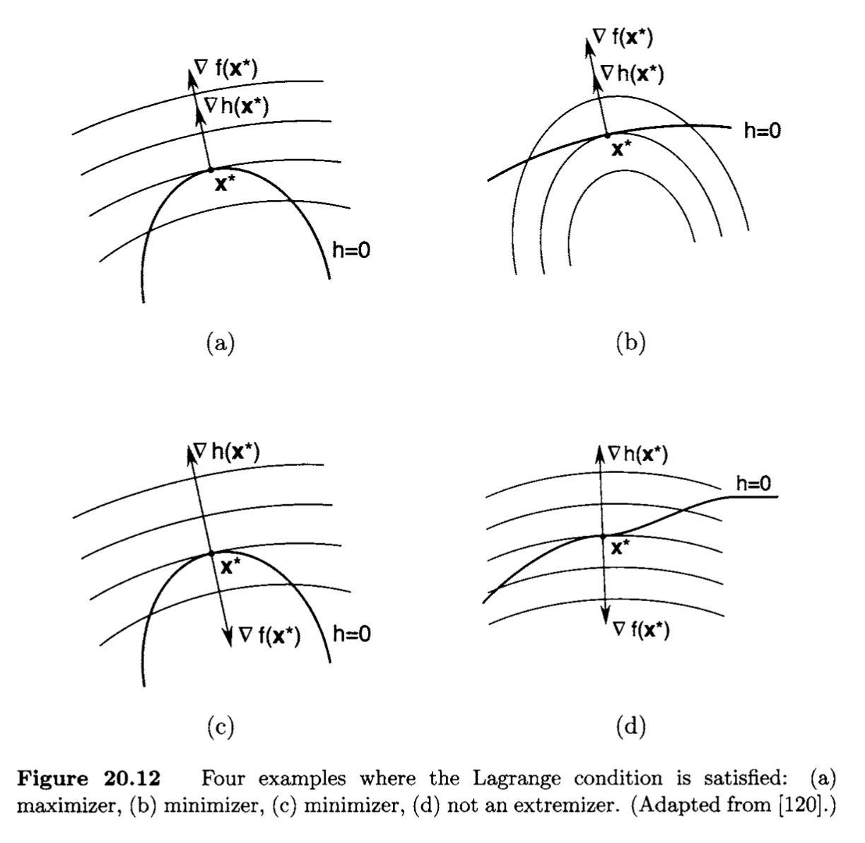
Note that the Lagrange condition is necessary but not sufficient. In Figure $20.12$ we illustrate a variety of points where the Lagrange condition is

Figure 20.11 Lagrange's theorem for $n=2, m=1$.

satisfied, including a case where the point is not an extremizer (neither a maximizer nor a minimizer).

We now generalize Lagrange's theorem for the case when $f: \mathbb{R}^{n} \rightarrow \mathbb{R}$ and $\boldsymbol{h}: \mathbb{R}^{n} \rightarrow \mathbb{R}^{m}, m \leq n$

Lagrange's Theorem

Let $x^{*}$ be a local minimizer (or maximizer) of $f: \mathbb{R}^{n} \rightarrow \mathbb{R}$, subject to $\boldsymbol{h}(\boldsymbol{x})=\mathbf{0}, \boldsymbol{h}: \mathbb{R}^{n} \rightarrow \mathbb{R}^{m}, m \leq n$. Assume that $\boldsymbol{x}^{*}$ is a regular point. Then, there exists $\boldsymbol{\lambda}^{*} \in \mathbb{R}^{m}$ such that

$$D f\left(\boldsymbol{x}^{*}\right)+\boldsymbol{\lambda}^{* \top} D \boldsymbol{h}\left(\boldsymbol{x}^{*}\right)=\mathbf{0}^{\top} .$$

Proof

We need to prove that

$$\nabla f\left(\boldsymbol{x}^{*}\right)=-D \boldsymbol{h}\left(\boldsymbol{x}^{*}\right)^{\top} \boldsymbol{\lambda}^{*}$$

for some $\boldsymbol{\lambda}^{*} \in \mathbb{R}^{m} ;$ that is, $\nabla f\left(\boldsymbol{x}^{*}\right) \in \mathcal{R}\left(D \boldsymbol{h}\left(\boldsymbol{x}^{*}\right)^{\top}\right)=N\left(\boldsymbol{x}^{*}\right)$. But by Lemma $20.1, N\left(\boldsymbol{x}^{*}\right)=T\left(\boldsymbol{x}^{*}\right)^{\perp}$. Therefore, it remains to show that $\nabla f\left(x^{*}\right) \in T\left(x^{*}\right)^{\perp}$

We proceed as follows. Suppose that

$$\boldsymbol{y} \in T\left(\boldsymbol{x}^{*}\right) .$$

Then, by Theorem $20.1$, there exists a differentiable curve $\{\boldsymbol{x}(t): t \in(a, b)\}$ such that for all $t \in(a, b)$,

$$\boldsymbol{h}(\boldsymbol{x}(t))=\mathbf{0},$$

and there exists $t^{*} \in(a, b)$ satisfying

$$\boldsymbol{x}\left(t^{*}\right)=\boldsymbol{x}^{*}, \quad \dot{\boldsymbol{x}}\left(t^{*}\right)=\boldsymbol{y} .$$

Now consider the composite function $\phi(t)=f(\boldsymbol{x}(t))$. Note that $t^{*}$ is a local minimizer of this function. By the first-order necessary condition for unconstrained local minimizers (see Theorem 6.1),

$$\frac{d \phi}{d t}\left(t^{*}\right)=0 .$$

Applying the chain rule yields

$$\frac{d \phi}{d t}\left(t^{*}\right)=D f\left(\boldsymbol{x}^{*}\right) \dot{\boldsymbol{x}}\left(t^{*}\right)=D f\left(\boldsymbol{x}^{*}\right) \boldsymbol{y}=\nabla f\left(\boldsymbol{x}^{*}\right)^{\top} \boldsymbol{y}=0 .$$

So all $\boldsymbol{y} \in T\left(\boldsymbol{x}^{*}\right)$ satisfy

$$\nabla f\left(x^{*}\right)^{\top} \boldsymbol{y}=0$$

Figure 20.13 Example where the Lagrange condition does not hold.

that is,

$$\nabla f\left(\boldsymbol{x}^{*}\right) \in T\left(\boldsymbol{x}^{*}\right)^{\perp}$$

This completes the proof.

Theorem (Second-Order Necessary Conditions)

Let $\boldsymbol{x}^{*}$ be a local minimizer of $f: \mathbb{R}^{n} \rightarrow \mathbb{R}$ subject to $\boldsymbol{h}(\boldsymbol{x})=\mathbf{0}, \boldsymbol{h}: \mathbb{R}^{n} \rightarrow \mathbb{R}^{m}, m \leq n$, and $f, \boldsymbol{h} \in \mathcal{C}^{2}$. Suppose that $\boldsymbol{x}^{*}$ is regular. Then, there exists $\boldsymbol{\lambda}^{*} \in \mathbb{R}^{m}$ such that:

1. $D \boldsymbol{f}\left(\boldsymbol{x}^{*}\right)+\boldsymbol{\lambda}^{* \top} D \boldsymbol{h}\left(\boldsymbol{x}^{*}\right)=\mathbf{0}^{\top}$.

2. For all $\boldsymbol{y} \in T\left(\boldsymbol{x}^{*}\right)$, we have $\boldsymbol{y}^{\top} \boldsymbol{L}\left(\boldsymbol{x}^{*}, \boldsymbol{\lambda}^{*}\right) \boldsymbol{y} \geq 0$.

Proof. The existence of $\boldsymbol{\lambda}^{*} \in \mathbb{R}^{m}$ such that $D f\left(\boldsymbol{x}^{*}\right)+\boldsymbol{\lambda}^{* \top} D \boldsymbol{h}\left(\boldsymbol{x}^{*}\right)=\mathbf{0}^{\top}$ follows from Lagrange's theorem. It remains to prove the second part of the result. Suppose that $\boldsymbol{y} \in T\left(\boldsymbol{x}^{*}\right)$; that is, $\boldsymbol{y}$ belongs to the tangent space to $S=\left\{\boldsymbol{x} \in \mathbb{R}^{n}: \boldsymbol{h}(\boldsymbol{x})=\mathbf{0}\right\}$ at $\boldsymbol{x}^{*}$. Because $\boldsymbol{h} \in \mathcal{C}^{2}$, following the argument of Theorem 20.1, there exists a twice-differentiable curve $\{\boldsymbol{x}(t): t \in(a, b)\}$ on $S$ such that

$$\boldsymbol{x}\left(t^{*}\right)=x^{*}, \quad \dot{x}\left(t^{*}\right)=\boldsymbol{y}$$

for some $t^{*} \in(a, b)$. Observe that by assumption, $t^{*}$ is a local minimizer of the function $\phi(t)=f(\boldsymbol{x}(t))$. From the second-order necessary condition for unconstrained minimization (see Theorem 6.2), we obtain

$$\frac{d^{2} \phi}{d t^{2}}\left(t^{*}\right) \geq 0 \text {. }$$

Using the formula

$$\frac{d}{d t}\left(\boldsymbol{y}(t)^{\top} \boldsymbol{z}(t)\right)=\boldsymbol{z}(t)^{\top} \frac{d \boldsymbol{y}}{d t}(t)+\boldsymbol{y}(t)^{\top} \frac{d \boldsymbol{z}}{d t}(t)$$

and applying the chain rule yields

$$\begin{aligned} \frac{d^{2} \phi}{d t^{2}}\left(t^{*}\right) &=\frac{d}{d t}\left[D f\left(\boldsymbol{x}\left(t^{*}\right)\right) \dot{\boldsymbol{x}}\left(t^{*}\right)\right] \\ &=\dot{\boldsymbol{x}}\left(t^{*}\right)^{\top} \boldsymbol{F}\left(\boldsymbol{x}^{*}\right) \dot{\boldsymbol{x}}\left(t^{*}\right)+D f\left(\boldsymbol{x}^{*}\right) \ddot{\boldsymbol{x}}\left(t^{*}\right) \\ &=\boldsymbol{y}^{\top} \boldsymbol{F}\left(\boldsymbol{x}^{*}\right) \boldsymbol{y}+D f\left(\boldsymbol{x}^{*}\right) \ddot{\boldsymbol{x}}\left(t^{*}\right) \geq 0 . \end{aligned}$$

Because $\boldsymbol{h}(\boldsymbol{x}(t))=\mathbf{0}$ for all $t \in(a, b)$, we have

$$\frac{d^{2}}{d t^{2}} \boldsymbol{\lambda}^{* \top} \boldsymbol{h}(\boldsymbol{x}(t))=0 .$$

Thus, for all $t \in(a, b)$,

$$\begin{aligned} \frac{d^{2}}{d t^{2}} \boldsymbol{\lambda}^{* \top} \boldsymbol{h}(\boldsymbol{x}(t)) &=\frac{d}{d t}\left[\boldsymbol{\lambda}^{* \top} \frac{d}{d t} \boldsymbol{h}(\boldsymbol{x}(t))\right] \\ &=\frac{d}{d t}\left[\sum_{k=1}^{m} \lambda_{k}^{*} \frac{d}{d t} h_{k}(\boldsymbol{x}(t))\right] \\ &=\frac{d}{d t}\left[\sum_{k=1}^{m} \lambda_{k}^{*} D h_{k}(\boldsymbol{x}(t)) \dot{\boldsymbol{x}}(t)\right] \\ &=\sum_{k=1}^{m} \lambda_{k}^{*} \frac{d}{d t}\left(D h_{k}(\boldsymbol{x}(t)) \dot{\boldsymbol{x}}(t)\right) \\ &=\sum_{k=1}^{m} \lambda_{k}^{*}\left[\dot{\boldsymbol{x}}(t)^{\top} \boldsymbol{H}_{k}(\boldsymbol{x}(t)) \dot{\boldsymbol{x}}(t)+D h_{k}(\boldsymbol{x}(t)) \ddot{\boldsymbol{x}}(t)\right] \\ &=\dot{\boldsymbol{x}}^{\top}(t)\left[\boldsymbol{\lambda}^{*} \boldsymbol{H}(\boldsymbol{x}(t))\right] \dot{\boldsymbol{x}}(t)+\boldsymbol{\lambda}^{* \top} D \boldsymbol{h}(\boldsymbol{x}(t)) \ddot{\boldsymbol{x}}(t) \\ &=0 . \end{aligned}$$

In particular, the above is true for $t=t^{*}$; that is,

$$\boldsymbol{y}^{\top}\left[\boldsymbol{\lambda}^{*} \boldsymbol{H}\left(\boldsymbol{x}^{*}\right)\right] \boldsymbol{y}+\boldsymbol{\lambda}^{* \top} D \boldsymbol{h}\left(\boldsymbol{x}^{*}\right) \ddot{\boldsymbol{x}}\left(t^{*}\right)=0 .$$

Adding this equation to the inequality

$$\boldsymbol{y}^{\top} \boldsymbol{F}\left(\boldsymbol{x}^{*}\right) \boldsymbol{y}+D f\left(\boldsymbol{x}^{*}\right) \ddot{\boldsymbol{x}}\left(t^{*}\right) \geq 0$$

yields

$$\boldsymbol{y}^{\top}\left(\boldsymbol{F}\left(\boldsymbol{x}^{*}\right)+\left[\boldsymbol{\lambda}^{*} \boldsymbol{H}\left(\boldsymbol{x}^{*}\right)\right]\right) \boldsymbol{y}+\left(D f\left(\boldsymbol{x}^{*}\right)+\boldsymbol{\lambda}^{* \top} D \boldsymbol{h}\left(\boldsymbol{x}^{*}\right)\right) \ddot{\boldsymbol{x}}\left(t^{*}\right) \geq 0 .$$

But, by Lagrange's theorem, $D f\left(x^{*}\right)+\lambda^{* \top} D \boldsymbol{h}\left(x^{*}\right)=\mathbf{0}^{\top}$. Therefore,

$$\boldsymbol{y}^{\top}\left(\boldsymbol{F}\left(\boldsymbol{x}^{*}\right)+\left[\boldsymbol{\lambda}^{*} \boldsymbol{H}\left(\boldsymbol{x}^{*}\right)\right]\right) \boldsymbol{y}=\boldsymbol{y}^{\top} \boldsymbol{L}\left(\boldsymbol{x}^{*}, \boldsymbol{\lambda}^{*}\right) \boldsymbol{y} \geq 0,$$

which proves the result.

Observe that $\boldsymbol{L}(\boldsymbol{x}, \boldsymbol{\lambda})$ plays a similar role as the Hessian matrix $\boldsymbol{F}(\boldsymbol{x})$ of the objective function $f$ did in the unconstrained minimization case. However, we now require that $\boldsymbol{L}\left(\boldsymbol{x}^{*}, \boldsymbol{\lambda}^{*}\right) \geq 0$ only on $T\left(\boldsymbol{x}^{*}\right)$ rather than on $\mathbb{R}^{n}$.

The conditions above are necessary, but not sufficient, for a point to be a local minimizer. We now present, without a proof, sufficient conditions for a point to be a strict local minimizer.

Theorem (Second-Order Sufficient Conditions)

Suppose that $f, \boldsymbol{h} \in \mathcal{C}^{2}$ and there exists a point $\boldsymbol{x}^{*} \in \mathbb{R}^{n}$ and $\boldsymbol{\lambda}^{*} \in \mathbb{R}^{m}$ such that:

1. $D f\left(\boldsymbol{x}^{*}\right)+\boldsymbol{\lambda}^{* \top} D \boldsymbol{h}\left(\boldsymbol{x}^{*}\right)=\mathbf{0}^{\top}$.
2. For all $\boldsymbol{y} \in T\left(\boldsymbol{x}^{*}\right), \boldsymbol{y} \neq \mathbf{0}$, we have $\boldsymbol{y}^{\top} \boldsymbol{L}\left(\boldsymbol{x}^{*}, \boldsymbol{\lambda}^{*}\right) \boldsymbol{y}>0$. Then, $\boldsymbol{x}^{*}$ is a strict local minimizer of $f$ subject to $\boldsymbol{h}(\boldsymbol{x})=\mathbf{0}$.