Duality

Suppose that we are given a linear programming problem of the form

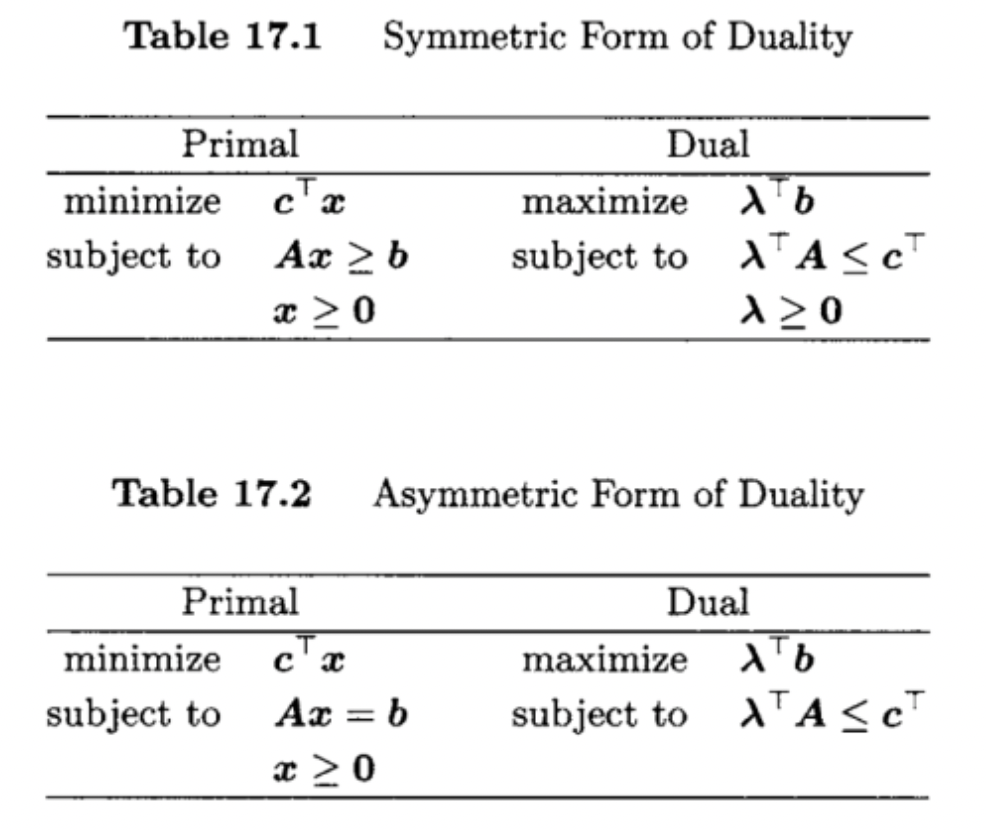
$$\begin{array}{ll}\text { minimize } & \boldsymbol{c}^{\top} \boldsymbol{x} \\ \text { subject to } & \boldsymbol{A}\boldsymbol{x} \geq \boldsymbol{b} \\ & \boldsymbol{x} \geq \boldsymbol{0} .\end{array}$$

We refer to the above as the primal problem. We define the corresponding dual problem as

$$\begin{array}{ll}\text { maximize } & \boldsymbol{\lambda}^{\top} \boldsymbol{b} \\ \text { subject to } & \boldsymbol{\lambda}^{\top} \boldsymbol{A} \leq \boldsymbol{c}^{\top} \\ & \boldsymbol{\lambda} \geq \boldsymbol{0} .\end{array}$$

We refer to the variable $\boldsymbol{\lambda} \in \mathbb{R}^m$ as the dual vector. Note that the cost vector $\boldsymbol{c}$ in the primal has moved to the constraints in the dual. The vector $\boldsymbol{b}$ on the righthand side of $\boldsymbol{A} \boldsymbol{x} \geq \boldsymbol{b}$ becomes part of the cost in the dual. Thus, the roles of $\boldsymbol{b}$ and $\boldsymbol{c}$ are reversed. The form of duality defined above is called the symmetric form of duality.

Note that the dual of the dual problem is the primal problem.

In summary:

Properties of Dual Problems

Lemma 1 (Weak Duality Lemma)

Suppose that $\boldsymbol{x}$ and $\boldsymbol{\lambda}$ are feasible solutions to primal and dual LP problems, respectively (either in the symmetric or asymmetric form). Then, $\boldsymbol{c}^{\top} \boldsymbol{x} \geq \boldsymbol{\lambda}^{\top} \boldsymbol{b}$.

Proof

We prove this lemma only for the asymmetric form of duality. The proof for the symmetric form involves only a slight modification. Because $\boldsymbol{x}$ and $\boldsymbol{\lambda}$ are feasible, we have $\boldsymbol{A x}=\boldsymbol{b}, \boldsymbol{x} \geq \boldsymbol{0}$, and $\boldsymbol{\lambda}^{\top} \boldsymbol{A} \leq \boldsymbol{c}^{\top}$. Postmultiplying both sides of the inequality $\boldsymbol{\lambda}^{\top} \boldsymbol{A} \leq \boldsymbol{c}^{\top}$ by $\boldsymbol{x} \geq \boldsymbol{0}$ yields $\boldsymbol{\lambda}^{\top} \boldsymbol{A x} \leq \boldsymbol{c}^{\top}$ $\boldsymbol{x}$. But $\boldsymbol{A x}=\boldsymbol{b}$, hence $\boldsymbol{\lambda}^{\top} \boldsymbol{b} \leq \boldsymbol{c}^{\top} \boldsymbol{x}$. The weak duality lemma states that a feasible solution to either problem yields a bound on the optimal cost of the other problem. The cost in the dual is never above the cost in the primal. In particular, the optimal cost of the dual is less than or equal to the optimal cost of the primal, that is, "maximum $\leq$ minimum." Hence, if the cost of one of the problems is unbounded, then the other problem has no feasible solution. In other words, if "minimum $=-\infty$ " or "maximum $=$ $+\infty$," then the feasible set in the other problem must be empty.

Theorem 1

Suppose that $\boldsymbol{x}_0$ and $\boldsymbol{\lambda}_0$ are feasible solutions to the primal and dual, respectively (either in symmetric or asymmetric form). If $\boldsymbol{c}^{\top} \boldsymbol{x}_0=\boldsymbol{\lambda}_0{ }^{\top} \boldsymbol{b}$, then $\boldsymbol{x}_0$ and $\boldsymbol{\lambda}_0$ are optimal solutions to their respective problems.

Proof

Let $\boldsymbol{x}$ be an arbitrary feasible solution to the primal problem. Because $\boldsymbol{\lambda}_0$ is a feasible solution to the dual, by the weak duality lemma, $\boldsymbol{c}^{\top} \boldsymbol{x} \geq \boldsymbol{\lambda}_0^{\top} \boldsymbol{b}$. So, if $\boldsymbol{c}^{\top}\boldsymbol{x}_0=\boldsymbol{\lambda}_0^{\top} \boldsymbol{b}$, then $c^{\top} \boldsymbol{x}_0=\boldsymbol{\lambda}_0^{\top} \boldsymbol{b} \leq \boldsymbol{c}^{\top} \boldsymbol{x}$. Hence, $\boldsymbol{x}_0$ is optimal for the primal.

On the other hand, let $\boldsymbol{\lambda}$ be an arbitrary feasible solution to the dual problem. Because $\boldsymbol{x}_0$ is a feasible solution to the primal, by the weak duality lemma, $\boldsymbol{c}^{\top} \boldsymbol{x}_0 \geq \boldsymbol{\lambda}^{\top} \boldsymbol{b}$. Therefore, if $\boldsymbol{c}^{\top} \boldsymbol{x}_0=\boldsymbol{\lambda}_0^{\top} \boldsymbol{b}$, then $\boldsymbol{\lambda}^{\top} \boldsymbol{b} \leq \boldsymbol{c}^{\top} \boldsymbol{x}_0=\boldsymbol{\lambda}_0^{\top} \boldsymbol{b}$. Hence, $\boldsymbol{\lambda}_0$ is optimal for the dual.

We can interpret Theorem 1 as follows. The primal seeks to minimize its cost, and the dual seeks to maximize its cost. Because the weak duality lemma states that "maximum $\leq$ minimum," each problem "seeks to reach the other." When their costs are equal for a pair of feasible solutions, both solutions are optimal, and we have “maximum = minimum.” It turns out that the converse of Theorem 1 is also true, that is, “maximum = minimum” always holds. In fact, we can prove an even stronger result, known as the duality theorem.

Theorem 2 (Duality Theorem)

If the primal problem (either in symmetric or asymmetric form) has an optimal solution, then so does the dual, and the optimal values of their respective objective functions are equal.

Proof

We first prove the result for the asymmetric form of duality. Assume that the primal has an optimal solution. Then, by the fundamental theorem of LP, there exists an optimal basic feasible solution. As is our usual notation, let $\boldsymbol{B}$ be the matrix of the corresponding $m$ basic columns, $\boldsymbol{D}$ the matrix of the $n-m$ non-basic columns, $\boldsymbol{c}_{\boldsymbol{B}}$ the vector of elements of $\boldsymbol{c}$ corresponding to basic variables, $\boldsymbol{c}_{\boldsymbol{D}}$ the vector of elements of $\boldsymbol{c}$ corresponding to nonbasic variables, and $\boldsymbol{r}_D$ the vector of reduced cost coefficients. Then, by the Theorem presented in the LP section,

$$\begin{gather*} \boldsymbol{r}_D^{\top}=\boldsymbol{c}_{\boldsymbol{D}}^{\top}-\boldsymbol{c}_{\boldsymbol{B}}^{\top} \boldsymbol{B}^{-1} \boldsymbol{D} \geq \boldsymbol{0}^{\top}. \end{gather*}$$

Hence,

$$\begin{gather*} \boldsymbol{c}_{\boldsymbol{B}}^{\top}\boldsymbol{B}^{-1}\boldsymbol{D}\leq \boldsymbol{c}_{\boldsymbol{D}}^{\top}. \end{gather*}$$

Define

$$\begin{gather*} \boldsymbol{\lambda}^{\top} = \boldsymbol{c}_{\boldsymbol{B}}^{\top}\boldsymbol{B}^{-1}. \end{gather*}$$

Then,

$$\begin{gather*} \boldsymbol{c}_{\boldsymbol{B}}^{\top}\boldsymbol{B}^{-1}\boldsymbol{D} = \boldsymbol{\lambda}^{\top}\boldsymbol{D} \leq \boldsymbol{c}_{\boldsymbol{D}}^{\top} \end{gather*}$$

We claim that $\boldsymbol{\lambda}$ is a feasible solution to the dual. To see this, assume for convenience (and without loss of generality) that the basic columns are the first $m$ columns of $\boldsymbol{A}$. Then,

$$\begin{gather*} \boldsymbol{\lambda}^{\top} \boldsymbol{A}=\boldsymbol{\lambda}^{\top}[\boldsymbol{B}, \boldsymbol{D}]=\left[\boldsymbol{c}_B^{\top}, \boldsymbol{\lambda}^{\top} \boldsymbol{D}\right] \leq\left[\boldsymbol{c}_B^{\top}, \boldsymbol{c}_D^{\top}\right]=\boldsymbol{c}^{\top}. \end{gather*}$$

Hence, $\boldsymbol{\lambda}^{\top} \boldsymbol{A} \leq \boldsymbol{c}^{\top}$ and thus $\boldsymbol{\lambda}^{\top}=\boldsymbol{c}_B \boldsymbol{B}^{-1}$ is feasible. We claim that $\boldsymbol{\lambda}$ is also an optimal feasible solution to the dual. To see this, note that

$$\begin{gather*} \boldsymbol{\lambda}^{\top} \boldsymbol{b}=\boldsymbol{c}_B^{\top} \boldsymbol{B}^{-1} \boldsymbol{b}=\boldsymbol{c}_B^{\top} \boldsymbol{x}_B. \end{gather*}$$

Thus, by Theorem 1, $\boldsymbol{\lambda}$ is optimal.

We now prove the symmetric case. First, we convert the primal problem for the symmetric form into the equivalent standard form by adding surplus variables:

$$\begin{align*} \operatorname{minimize} & \left[\boldsymbol{c}^{\top}, \boldsymbol{0}^{\top}\right]\left[\begin{array}{l}\boldsymbol{x} \\ \boldsymbol{y}\end{array}\right] \\ \text{subject to } & [\boldsymbol{A},-\boldsymbol{I}]\left[\begin{array}{l}\boldsymbol{x} \\ \boldsymbol{y}\end{array}\right]=\boldsymbol{b} \\ & \left[\begin{array}{l}\boldsymbol{x} \\ \boldsymbol{y}\end{array}\right] \geq \boldsymbol{0}. \end{align*}$$

Note that $\boldsymbol{x}$ is optimal for the original primal problem if and only if $\left[\boldsymbol{x}^{\top},(\boldsymbol{A}\boldsymbol{x}-\boldsymbol{b})\right.$ $\left.{ }^{\top}\right]^{\top}$ is optimal for the primal in standard form. The dual to the primal in standard form is equivalent to the dual to the original primal in symmetric form. Therefore, the result above for the asymmetric case applies also to the symmetric case. This completes the proof.

Theorem 3 (Complementary Slackness Condition)

The feasible solutions $\boldsymbol{x}$ and $\boldsymbol{\lambda}$ to a dual pair of problems (either in symmetric or asymmetric form) are optimal if and only if:

1. $\left(\boldsymbol{c}^{\top}-\boldsymbol{\lambda}^{\top} \boldsymbol{A}\right) \boldsymbol{x}=0$.
2. $\boldsymbol{\lambda}^{\top}(\boldsymbol{A} \boldsymbol{x}-\boldsymbol{b})=0$.

Proof

We first prove the result for the asymmetric case. Note that condition 2 holds trivially for this case. Therefore, we consider only condition 1.

$\Rightarrow$ : If the two solutions are optimal, then by Theorem 2, $\boldsymbol{c}^{\top} \boldsymbol{x}=\lambda^{\top} \boldsymbol{b}$. Because $\boldsymbol{A} \boldsymbol{x}=\boldsymbol{b}$, we also have $\left(\boldsymbol{c}^{\top}-\boldsymbol{\lambda}^{\top} \boldsymbol{A}\right) \boldsymbol{x}=0$.

$\Leftarrow$ If $\left(\boldsymbol{c}^{\top}-\boldsymbol{\lambda}^{\top} \boldsymbol{A}\right) \boldsymbol{x}=0$, then $\boldsymbol{c}^{\top} \boldsymbol{x}=\boldsymbol{\lambda}^{\top} \boldsymbol{A} \boldsymbol{x}=\boldsymbol{\lambda}^{\top} \boldsymbol{b}$. Therefore, by Theorem 1, $\boldsymbol{x}$ and $\boldsymbol{\lambda}$ are optimal.

We now prove the result for the symmetric case.

$\Rightarrow$ We first show condition 1. If the two solutions are optimal, then by Theorem 2, $\boldsymbol{c}^{\top} \boldsymbol{x}=\boldsymbol{\lambda}^{\top} \boldsymbol{b}$. Because $\boldsymbol{A x} \geq \boldsymbol{b}$ and $\boldsymbol{\lambda} \geq \boldsymbol{0}$, we have

$$\begin{align*} \left(\boldsymbol{c}^{\top}-\boldsymbol{\lambda}^{\top} \boldsymbol{A}\right) \boldsymbol{x} & =\boldsymbol{c}^{\top} \boldsymbol{x}-\boldsymbol{\lambda}^{\top} \boldsymbol{A} \boldsymbol{x} \\ & = \boldsymbol{\lambda}^{\top} \boldsymbol{b}-\boldsymbol{\lambda}^{\top} \boldsymbol{A} \boldsymbol{x} \\ & = \boldsymbol{\lambda}^{\top}(\boldsymbol{b}-\boldsymbol{A} \boldsymbol{x}) \leq 0. \end{align*}$$

On the other hand, since $\boldsymbol{\lambda}^{\top} \boldsymbol{A} \leq \boldsymbol{c}^{\top}$ and $\boldsymbol{x} \geq \boldsymbol{0}$, we have $\left(\boldsymbol{c}^{\top}-\boldsymbol{\lambda}^{\top} \boldsymbol{A}\right) \boldsymbol{x} \geq 0$. Hence, $\left(\boldsymbol{c}^{\top}\right.$$\left.-\boldsymbol{\lambda}^{\top} \boldsymbol{A}\right) \boldsymbol{x}=0$. To show condition 2, note that since $\boldsymbol{A} \boldsymbol{x} \geq \boldsymbol{b}$ and $\boldsymbol{\lambda} \geq \mathbf{0}$, we have $\boldsymbol{\lambda}^{\top}$ ( $\boldsymbol{A x}-\boldsymbol{b}) \geq 0$. On the other hand, since $\boldsymbol{\lambda}^{\top} \boldsymbol{A} \leq \boldsymbol{c}^{\top}$ and $\boldsymbol{x} \geq \mathbf{0}$, we have $\boldsymbol{\lambda}^{\top}(\boldsymbol{A} \boldsymbol{x}-\boldsymbol{b})=$ $\left(\boldsymbol{\lambda}^{\top} \boldsymbol{A}-\boldsymbol{c}^{\top}\right) \boldsymbol{x} \leq 0$.

$\Leftarrow$ Combining conditions 1 and 2, we get $\boldsymbol{c}^{\top} \boldsymbol{x}=\boldsymbol{\lambda}^{\top} \boldsymbol{A} \boldsymbol{x}=\boldsymbol{\lambda}^{\top} \boldsymbol{b}$. Hence, by Theorem 1, $\boldsymbol{x}$ and $\boldsymbol{\lambda}$ are optimal.

Note that if $\boldsymbol{x}$ and $\boldsymbol{\lambda}$ are feasible solutions for the dual pair of problems, we can write condition 1 , that is, $\left(\boldsymbol{c}^{\top}-\boldsymbol{\lambda}^{\top} \boldsymbol{A}\right) \boldsymbol{x}=0$, as " $\boldsymbol{x}_i>0$ implies that $\boldsymbol{\lambda} \boldsymbol{a}_i=\boldsymbol{c}_{\boldsymbol{i}}, i=1$, $\ldots, n$," that is, for any component of $\boldsymbol{x}$ that is positive, the corresponding constraint for the dual must be an equality at $\boldsymbol{\lambda}$. Also, observe that the statement " $\boldsymbol{x}_i>0$ implies that $\boldsymbol{\lambda}^{\top} \boldsymbol{a}_i=\boldsymbol{c}_i$ " is equivalent to "$\boldsymbol{\lambda}^{\top} \boldsymbol{a}_i<\boldsymbol{c}_i$ implies that $\boldsymbol{x}_i=0$." A similar representation can be written for condition 2 .

Consider the asymmetric form of duality. Recall that for the case of an optimal basic feasible solution $\boldsymbol{x}, \boldsymbol{r}^{\top}=\boldsymbol{c}^{\top}-\boldsymbol{\lambda}^{\top} \boldsymbol{A}$ is the vector of reduced cost coefficients. Therefore, in this case, the complementary slackness condition can be written as $\boldsymbol{r}^{\top} \boldsymbol{x}=0$.