Monte Carlo Methods

What's Monte Carlo?

The term Monte Carlo is often used more broadly for any estimation method that relies on repeated random sampling. In RL Monte Carlo methods allow us to estimate values directly from experience, from sequences of states, actions and rewards. Learning from experience is striking because the agent can accurately estimate a value function without prior knowledge of the environment dynamics.
To use a pure Dynamic Programming approach, the agent needs to know the environment's transition probabilities.

• In some problems, we do not know the environment's transition probabilities
• The computation can be error-prone and tedious For example, imagine rolling a die. With the help of Monte Carlo Methods, we can estimate values by averaging over a large number of random samples.

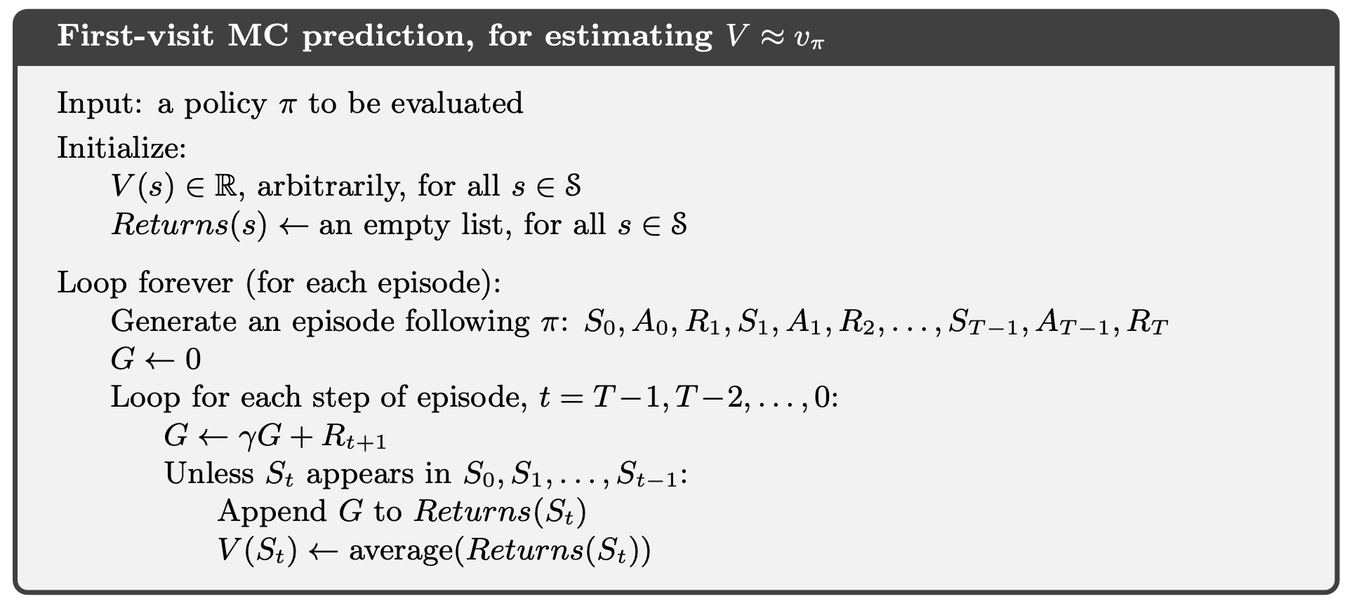
Monte Carlo Prediction

In particular, suppose we wish to estimate $v_\pi(s)$, the value of a state $s$ under policy $\pi$, given a set of episodes obtained by following $\pi$ and passing through $s$. Each occurrence of state $s$ in an episode is called a visit to $s$. Of course, $s$ may be visited multiple times in the same episode; let us call the first time it is visited in an episode the first visit to $s$. The first-visit $M C$ method estimates $v_\pi(s)$ as the average of the returns following first visits to $s$, whereas the every-visit $M C$ method averages the returns following all visits to $s$. We focus on the first-visit MC method here.

Monte Carlo Estimation of Action Values

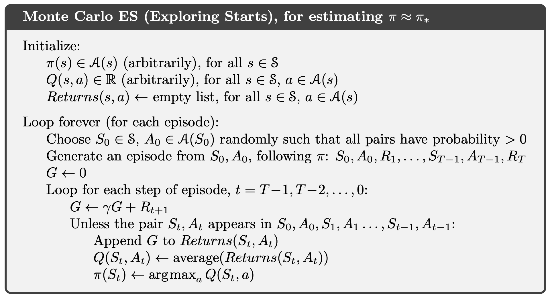
One serious complication arises when we do not visit every state, as can be the case if our policy is deterministic. If we do not visit states then we do not observe returns from these states and cannot estimate their value. We, therefore, need to maintain exploration of the state space. One way of doing so is stochastically selecting a state-action pair to start an episode, giving every state-action pair a non-zero probability of being selected. In this case, we are said to be utilizing exploring starts.

Monte Carlo Control

• Much like we did with value iteration, we do not need to fully evaluate the value function for a given policy in Monte Carlo control. Instead, we can merely move the value toward the correct value and then switch to policy improvement thereafter. It is natural to do this episodically i.e. evaluate the policy using one episode of experience, then act greedily w.r.t the previous value function to improve the policy in the next episode.
• If we use a deterministic policy for control, we must use exploring starts to ensure sufficient exploration. This creates the Monte Carlo ES algorithm.

Monte Carlo Control without Exploring Starts

• The only general way to ensure that all actions are selected infinitely often is for the agent to continue to select them. There are two approaches to ensuring this, resulting in what we call on-policy methods and off-policy methods. On-policy methods attempt to evaluate or improve the policy that is used to make decisions, whereas off-policy methods evaluate or improve a policy different from that used to generate the data.
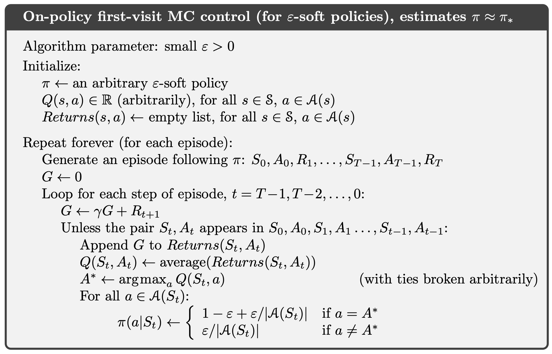
• In on-policy control methods, the policy is generally soft, meaning that $\pi(a|s) > 0$ for all $s \in S$ and all $a \in A(s)$, but gradually shifted closer and closer to a deterministic optimal policy.

$\varepsilon$-soft policies

The on-policy method we present in this section uses $\varepsilon$-greedy policies, meaning that most of the time they choose an action that has maximal estimated action value, but with probability $\varepsilon$ they instead select an action at random. That is, all nongreedy actions are given the minimal probability of selection, $\frac{\varepsilon}{|\mathcal{A}(s)|}$, and the remaining bulk of the probability, $1-\varepsilon+\frac{\varepsilon}{|\mathcal{A}(s)|}$, is given to the greedy action. The $\varepsilon$-greedy policies are examples of $\varepsilon$-soft policies, defined as policies for which $\pi(a \mid s) \geq \frac{\varepsilon}{|\mathcal{A}(s)|}$ for all states and actions, for some $\varepsilon>0$. Among $\varepsilon$-soft policies, $\varepsilon$-greedy policies are in some sense those that are closest to greedy.

That any $\varepsilon$-greedy policy with respect to $q_\pi$ is an improvement over any $\varepsilon$-soft policy $\pi$ is assured by the policy improvement theorem. Let $\pi^{\prime}$ be the $\varepsilon$-greedy policy. The conditions of the policy improvement theorem apply because for any $s \in \mathcal{S}$ :

$$\begin{aligned} q_\pi\left(s, \pi^{\prime}(s)\right) &=\sum_a \pi^{\prime}(a \mid s) q_\pi(s, a) \\ &=\frac{\varepsilon}{|\mathcal{A}(s)|} \sum_a q_\pi(s, a)+(1-\varepsilon) \max _a q_\pi(s, a) \\ & \geq \frac{\varepsilon}{|\mathcal{A}(s)|} \sum_a q_\pi(s, a)+(1-\varepsilon) \sum_a \frac{\pi(a \mid s)-\frac{\varepsilon}{|\mathcal{A}(s)|}}{1-\varepsilon} q_\pi(s, a) \end{aligned}$$

(the sum is a weighted average with nonnegative weights summing to 1 , and as such it must be less than or equal to the largest number averaged)

$$\begin{aligned} &=\frac{\varepsilon}{|\mathcal{A}(s)|} \sum_a q_\pi(s, a)-\frac{\varepsilon}{|\mathcal{A}(s)|} \sum_a q_\pi(s, a)+\sum_a \pi(a \mid s) q_\pi(s, a) \\ &=v_\pi(s) \end{aligned}$$

Thus, by the policy improvement theorem, $\pi^{\prime} \geq \pi$ (i.e., $v_{\pi^{\prime}}(s) \geq v_\pi(s)$, for all $\left.s \in \mathcal{S}\right)$. We now prove that equality can hold only when both $\pi^{\prime}$ and $\pi$ are optimal among the $\varepsilon$-soft policies, that is when they are better than or equal to all other $\varepsilon$-soft policies.

Off-policy Prediction via Importance Sampling

All learning control methods face a dilemma: They seek to learn action values conditional on subsequent optimal behavior, but they need to behave non-optimally in order to explore all actions (to find the optimal actions). How can they learn about the optimal policy while behaving according to an exploratory policy? The on-policy approach in the preceding section is actually a compromise-it learns action values not for the optimal policy, but for a near-optimal policy that still explores. A more straightforward approach is to use two policies, one that is learned about and that becomes the optimal policy, and one that is more exploratory and is used to generate behavior. The policy being learned about is called the target policy, and the policy used to generate behavior is called the behavior policy. In this case, we say that learning is from data "off" the target policy, and the overall process is termed off-policy learning.

In this section, we begin the study of off-policy methods by considering the prediction problem, in which both target and behavior policies are fixed. That is, suppose we wish to estimate $v_\pi$ or $q_\pi$, but all we have are episodes following another policy $b$, where $b \neq \pi$. In this case, $\pi$ is the target policy, $b$ is the behavior policy, and both policies are considered fixed and given.

In order to use episodes from $b$ to estimate values for $\pi$, we require that every action taken under $\pi$ is also taken, at least occasionally, under $b$. That is, we require that $\pi(a \mid s)>0$ implies $b(a \mid s)>0$. This is called the assumption of coverage. It follows from coverage that $b$ must be stochastic in states where it is not identical to $\pi$. The target policy $\pi$, on the other hand, maybe deterministic, and, in fact, this is a case of particular interest in control applications. In control, the target policy is typically the deterministic greedy policy with respect to the current estimate of the action-value function. This policy becomes a deterministic optimal policy while the behavior policy remains stochastic and more exploratory, for example, an $\varepsilon$-greedy policy. In this section, however, we consider the prediction problem, in which $\pi$ is unchanging and given.

Almost all off-policy methods utilize importance sampling, a general technique for estimating expected values under one distribution given samples from another. We apply importance sampling to off-policy learning by weighting returns according to the relative probability of their trajectories occurring under the target and behavior policies, called the importance-sampling ratio. Given a starting state $S_t$, the probability of the subsequent state-action trajectory, $A_t, S_{t+1}, A_{t+1}, \ldots, S_T$, occurring under any policy $\pi$ is

$$\begin{aligned} \operatorname{Pr} &\left\{A_t, S_{t+1}, A_{t+1}, \ldots, S_T \mid S_t, A_{t: T-1} \sim \pi\right\} \\ &=\pi\left(A_t \mid S_t\right) p\left(S_{t+1} \mid S_t, A_t\right) \pi\left(A_{t+1} \mid S_{t+1}\right) \cdots p\left(S_T \mid S_{T-1}, A_{T-1}\right) \\ &=\prod_{k=t}^{T-1} \pi\left(A_k \mid S_k\right) p\left(S_{k+1} \mid S_k, A_k\right) \end{aligned}$$

where $p$ here is the state-transition probability function defined by (3.4). Thus, the relative probability of the trajectory under the target and behavior policies (the importancesampling ratio) is

$$\rho_{t: T-1} \doteq \frac{\prod_{k=t}^{T-1} \pi\left(A_k \mid S_k\right) p\left(S_{k+1} \mid S_k, A_k\right)}{\prod_{k=t}^{T-1} b\left(A_k \mid S_k\right) p\left(S_{k+1} \mid S_k, A_k\right)}=\prod_{k=t}^{T-1} \frac{\pi\left(A_k \mid S_k\right)}{b\left(A_k \mid S_k\right)} .$$

Although the trajectory probabilities depend on the MDP's transition probabilities, which are generally unknown, they appear identically in both the numerator and denominator and thus cancel. The importance sampling ratio ends up depending only on the two policies and the sequence, not on the MDP.

Recall that we wish to estimate the expected returns (values) under the target policy, but all we have are returns $G_t$ due to the behavior policy. These returns have the wrong expectation $\mathbb{E}\left[G_t \mid S_t=s\right]=v_b(s)$ and so cannot be averaged to obtain $v_\pi$. This is where importance sampling comes in. The ratio $\rho_{t: T-1}$ transforms the returns to have the right expected value:

$$\mathbb{E}\left[\rho_{t: T-1} G_t \mid S_t=s\right]=v_\pi(s) .$$

Now we are ready to give a Monte Carlo algorithm that averages returns from a batch of observed episodes following policy $b$ to estimate $v_\pi(s)$. It is convenient here to number time steps in a way that increases across episode boundaries. That is, if the first episode of the batch ends in a terminal state at time 100, then the next episode begins at time $t=101$. This enables us to use time-step numbers to refer to particular steps in particular episodes. In particular, we can define the set of all time steps in which state $s$ is visited, denoted $\mathcal{T}(s)$. This is for an every-visit method; for a first-visit method, $\mathcal{T}(s)$ would only include time steps that were first visits to $s$ within their episodes. Also, let $T(t)$ denote the first time of termination following time $t$, and $G_t$ denote the return after $t$ up through $T(t)$. Then $\left\{G_t\right\}_{t \in \mathcal{T}(s)}$ are the returns that pertain to state $s$, and $\left\{\rho_{t: T(t)-1}\right\}_{t \in \mathcal{T}(s)}$ are the corresponding importance-sampling ratios. To estimate $v_\pi(s)$, we simply scale the returns by the ratios and average the results:

$$V(s) \doteq \frac{\sum_{t \in \mathcal{T}(s)} \rho_{t: T(t)-1} G_t}{|\mathcal{T}(s)|}$$

When importance sampling is done as a simple average in this way it is called ordinary importance sampling.

An important alternative is weighted importance sampling, which uses a weighted average, defined as

$$V(s) \doteq \frac{\sum_{t \in \mathcal{T}(s)} \rho_{t: T(t)-1} G_t}{\sum_{t \in \mathcal{T}(s)} \rho_{t: T(t)-1}},$$

or zero if the denominator is zero. However, these two methods are biased.

Incremental Implementation

Suppose we have a sequence of returns $G_1, G_2, \ldots, G_{n-1}$, all starting in the same state and each with a corresponding random weight $W_i$ (e.g., $\left.W_i=\rho_{t_i: T\left(t_i\right)-1}\right)$. We wish to form the estimate

$$V_n \doteq \frac{\sum_{k=1}^{n-1} W_k G_k}{\sum_{k=1}^{n-1} W_k}, \quad n \geq 2,$$

and keep it up-to-date as we obtain a single additional return $G_n$. In addition to keeping track of $V_n$, we must maintain for each state the cumulative sum $C_n$ of the weights given to the first $n$ returns. The update rule for $V_n$ is

$$V_{n+1} \doteq V_n+\frac{W_n}{C_n}\left[G_n-V_n\right], \quad n \geq 1,$$

and

$$C_{n+1} \doteq C_n+W_{n+1},$$

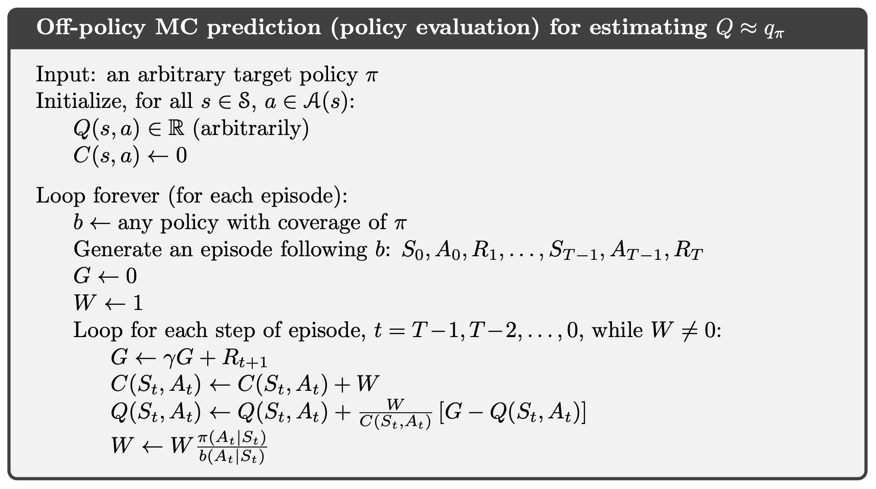
where $C_0 \doteq 0$ (and $V_1$ is arbitrary and thus need not be specified). The box on the next page contains a complete episode-by-episode incremental algorithm for Monte Carlo policy evaluation. The algorithm is nominally for the off-policy case, using weighted importance sampling, but applies as well to the on-policy case just by choosing the target and behavior policies as the same (in which case $(\pi=b), W$ is always 1). The approximation $Q$ converges to $q_\pi$ (for all encountered state-action pairs) while actions are selected according to a potentially different policy, $b$.

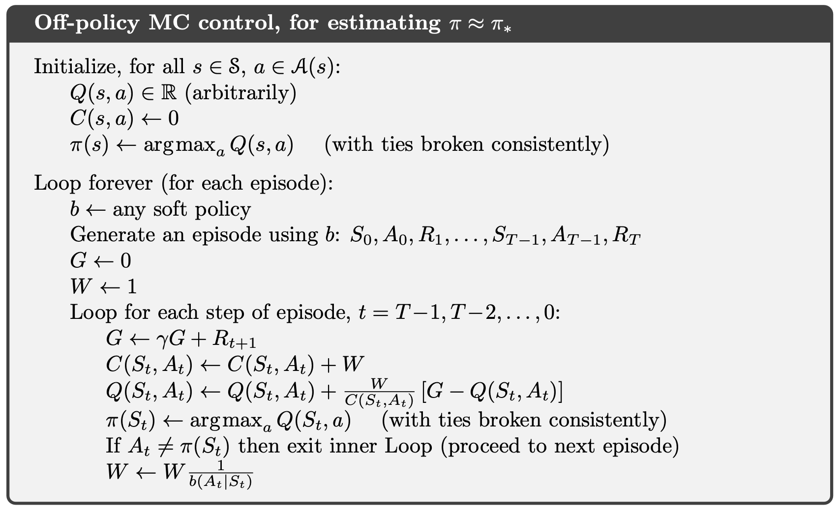
Off-policy Monte Carlo Control

Using incremental implementation (updates to the value function) and importance sampling we can now discuss the off-policy Monte Carlo control-the algorithm for obtaining optimal policy $\pi_*$ by using rewards obtained through behavior policy $b$. This works in much the same way as in previous sections; $b$ must be $\epsilon$-soft to ensure the entire state space is explored in the limit; updates are only made to our estimate for $q_\pi, Q$ if the sequence of states an actions produced by $b$ could have been produced by $\pi$. This algorithm is also based on GPI: we update our estimate of $Q$ using Equation 33, then update $\pi$ by acting greedily w.r.t to our value function. If this policy improvement changes our policy such that the trajectory we are in from $b$ no longer obeys our policy, then we exit the episode and start again.