Markov Decision Process

The Agent–Environment Interface

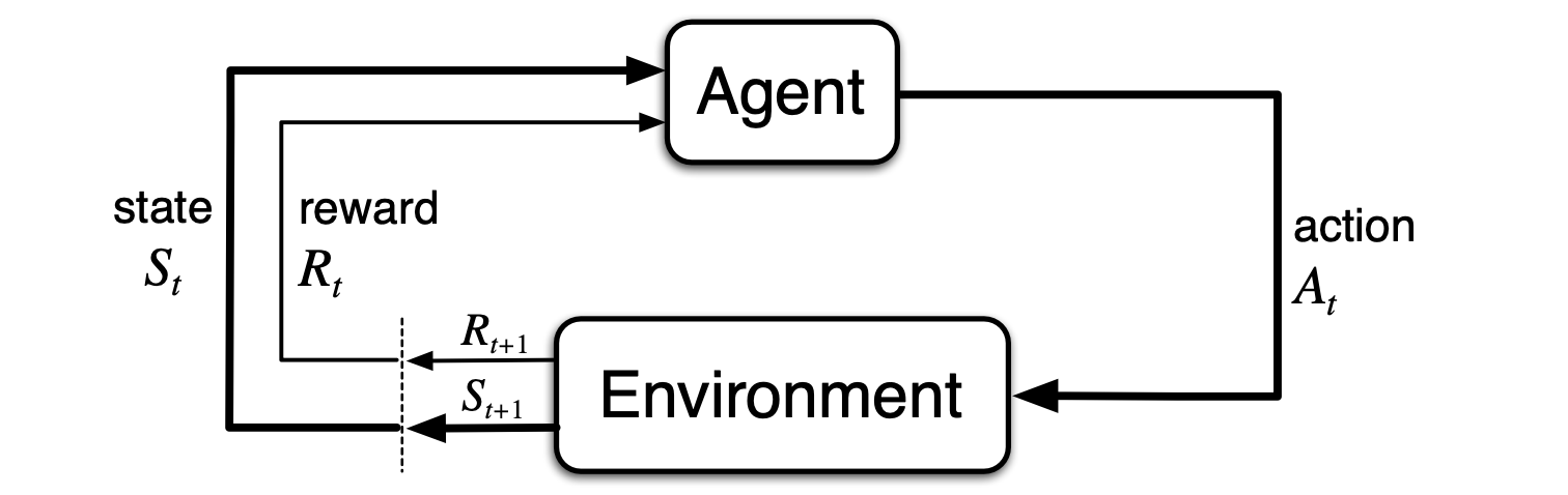
• At each time step the agent implements a mapping from states to probabilities of selecting a possible action. The mapping is called the agent's policy, denoted $\pi$, where $\pi (a|s)$ is the probability of the agent selecting action $a$ in state $s$.

• In general, actions can be any decision we want to learn how to make, and states can be any interpretation of the world that might inform those actions.

• The boundary between the agent and environment is much closer to the agent than is first intuitive. E.g. if we are controlling a robot, the voltages or stresses in its structure are part of the environment, not the agent. Indeed reward signals are part of the environment, despite very possibly being produced by the agent e.g. dopamine.

Markov Property

The future is independent of the past given the present.

• In contrast to normal causal processes, we would think that our expectation of the state and reward at the next timestep is a function of all previous states, rewards and actions, as follows:
  $$\begin{gather*} Pr\{R_{t+1}=r, S_{t+1}=s'|S_0, A_0, R-1, \cdots, S_{t-1}, A_{t-1}, R_t, S_t, A_t\} \end{gather*}$$
• If the state is Markov, however, then the state and reward right now completely characterize the history, and the above can be reduced to
  $$\begin{gather*} p(s', r|s, a) = Pr\{R_{t+1} = r, S_{t+1} = s'|S_t, A_t\} \end{gather*}$$
• Markov property is important in RL because decisions and values are assumed to be a function only of the current state.

Markov Decision Process (MDP)

From the four-argument dynamics function, p, one can compute anything else one might want to know about the environment, such as the state-transition probabilities,

$$\begin{gather*} p(s'|s, a) \doteq Pr\{S_t = s'|S_{t-1}=s, A_{t-1}=a\} = \sum_{r\in R}p(s', r|s, a). \end{gather*}$$

We can also compute the expected rewards for state–action pairs as a two-argument function $r : S \times A \to \mathbb{R}$:

$$\begin{gather*} r(s, a) \doteq \mathbb{E}[R_t|S_{t-1}=s, A_{t-1}=a] = \sum_{r\in R}\sum_{s'\in S}p(s', r|s, a), \end{gather*}$$

and the expected rewards for state–action–next-state triples as a three-argument function $r : S \times A \times S \to \mathbb{R}$,

$$\begin{gather*} r(s, a, s') \doteq \mathbb{E}[R_t|S_{t-1}=s, A_{t-1}=a, S_t = s'] = \sum_{r\in R}r{p(s', r|s, a) \over p(s'|s, a)}. \end{gather*}$$

Goals and Rewards

Reward Hypothesis

That all of what we mean by goals and purposes can be well thought of as the maximization of the expected value of the cumulative sum of a received scalar signal (called reward).

Return (Goal)

• In general, we seek to maximize the expected return, where the return, denoted Gt, is defined as some specific function of the reward sequence. In the simplest case, the return is the sum of the rewards:

  $$\begin{gather*} G_t \doteq R_{t+1}+R_{t+2}+R_{t+3}+\cdots +R_T, \end{gather*}$$

  where T is a final time step.

• This approach makes sense in applications that finish or are periodic. That is, the agent environment interaction breaks into episodes.

• We call these systems episodic tasks. e.g playing a board game and trips through a maze etc.

• Notation for state space in an episodic task varies from the conventional case $(s \in S)$ to $(s \in S^+)$

• The opposite, continuous applications are called continuing tasks. For these tasks, we use discounted returns to avoid a sum of returns going to infinity.

  $$\begin{gather*} G_t \doteq R_{t+1}+\gamma R_{t+2}+ \gamma^2R_{t+3}+\cdots = \sum_{k=0}^\infty \gamma^kR_{t+k+1}, 0 \le \gamma \le 1 \end{gather*}$$

  If the reward is a constant +1, then the return is

  $$\begin{gather*} G_t = \sum_{k=0}^\infty \gamma^k = {1\over 1-\gamma}. \end{gather*}$$

  Returns at successive time steps are related to each other in a way that is important for the theory and algorithms of reinforcement learning:

  $$\begin{gather*} G_t \doteq R_{t+1}+\gamma G_{t+1} \end{gather*}$$

  Alternatively, we can write

  $$\begin{gather*} G_t \doteq \sum_{k=t+1}^T \gamma^{k-t-1} R_k. \end{gather*}$$

Policies and Value Functions

Policy

A policy $\pi$ is a distribution over actions given states,

$$\begin{gather*} \pi(a|s) = \mathrm{P}[A_t = a | S_t = s] \end{gather*}$$

State Value Function

The value function of a state $s$ under a policy $\pi$, denoted $v_\pi (s)$, is the expected return when starting in $s$ and following $\pi$ thereafter. For MDPs, we can define $v_\pi$ formally by

$$\begin{gather*} v_\pi(s) \doteq \mathbb{E}_\pi[G_t | S_t = s] = \mathbb{E}_\pi[\sum_{k=0}^\infty \gamma^kR_{t+k+1} | S_t = s], \forall s \in S, \end{gather*}$$

where $\mathbb{E}_\pi [\cdot ]$ denotes the expected value of a random variable given that the agent follows policy $\pi$, and $t$ is any time step. Note that the value of the terminal state, if any, is always zero. We call the function $v_\pi$ the state-value function for policy $\pi$.
In recursive form (recall Bellman Equation):

$$\begin{align*} v_\pi(s) & \doteq \mathbb{E}_\pi[G_t | S_t = s] \\ & = \mathbb{E}_\pi[R_{t+1}+\gamma G_{t+1} | S_t = s] \\ & = \sum_a \pi(a|s)\sum_{s'}\sum_r p(s',r|s,a)\Big [r+\gamma\mathbb{E}[G_{t+1}|S_{t+1}=s']\Big ] \\ & = \sum_a \pi(a|s)\sum_{s',r} p(s',r|s,a)\Big [r+\gamma v_\pi(s')\Big ], \forall s \in S. \end{align*}$$

Action Value Function

Similarly, we define the value of taking action $a$ in state $s$ under a policy $\pi$, denoted $q_\pi(s,a)$, as the expected return starting from $s$, taking the action $a$, and thereafter following policy $\pi$:

$$\begin{gather*} q_\pi(s, a) \doteq \mathbb{E}_\pi[G_t | S_t = s, A_t = a] = \mathbb{E}_\pi[\sum_{k=0}^\infty \gamma^kR_{t+k+1} | S_t = s, A_t = a]. \end{gather*}$$

We call $q_\pi$ the action-value function for policy \pi.

Optimal Policies and Optimal Value Functions

The main objective of an RL algorithm is the best behavior an agent can take to maximize the goal.

• The optimal state-value function $v_{*}(s)$ is the maximum value function over all policies

  $$\begin{gather*} v_{*}(s) \doteq \max_{\pi} \ v_{\pi}(s), \forall s\in S. \end{gather*}$$

• The optimal action-value function $q_{*}(s,a)$ is the maximum action-value function over all policies

  $$\begin{gather*} q_{*}(s,a) \doteq \max_{\pi} \ q_{\pi}(s,a), \forall s\in S, a \in A(s). \end{gather*}$$

• For the state–action pair $(s,a)$, this function gives the expected return for taking action $a$ in state $s$ and thereafter following an optimal policy. Thus, we can write $q_*$ in terms of $v_*$ as follows:

$$\begin{gather*} q_{*}(s,a) = \mathbb{E}[R_{t+1}+\gamma v_*(S_{t+1})|S_t=s,A_t=a]. \end{gather*}$$

Extensions of MDPs

• Infinite and Continuous MDPs
• Partially observable MDPs
• Undiscounted, average reward MDPs