Dynamic Programming

---

Discrete-time Optimal Control Problems

We will next study the method of dynamic programming to solve optimal control problems. Dynamic programming relies on the principle of optimality that was developed by Richard Bellman around 1958 when he was working in RAND cooperation. Since then dynamic programming has been heavily used in computer science, operations research, control, and robotics among other domains.

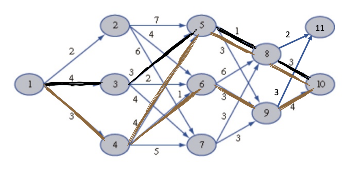
To understand what dynamic programming is, we will consider the following simple example where we are interested in taking a path from $A$ to $B$ with minimum cost.

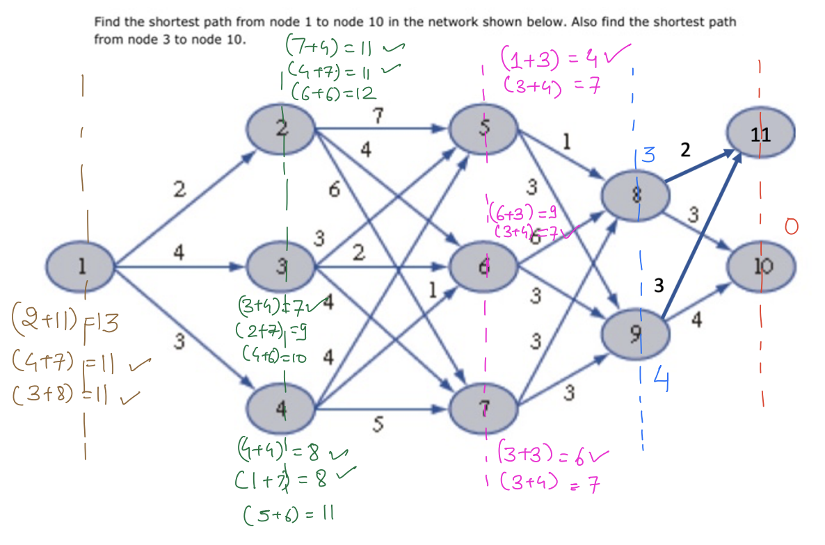
There are 3 optimal paths from node 1 to node 10, all with equal costs.

There are a few important things to note here about dynamic programming:

• DP gives you the optimal path from all nodes to node 10. So we get the optional solution for the intermediate nodes for free.

• Because it explores all intermediate nodes, it provides us with a globally optimal solution to our problem.

• DP gives us significant computational savings over forward computation/shooting methods.

Principle of Optimality

Now, let's try to understand the underlying mathematical principle based on the above example. DP relies on the principle of optimality: To understand the principle of optimality:

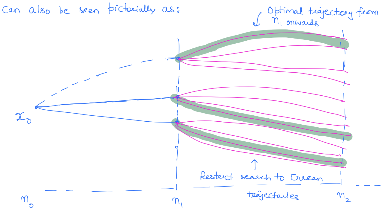
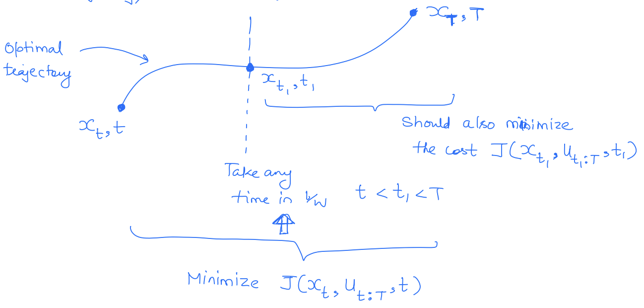
In an optimal sequence of decisions or choices, each subsequence must also be optimal. Thus, if we take any state along the optimal state trajectory, then the remaining sub-trajectory is also optimal."

In the above example, if I take any intermediate node along the optimal route, I take the most optimal route from that intermediate node to the destination node. This can also be seen pictorially as:

We can also write down the principle of optimality in a mathematical way. Our goal in the above route planning problem is to minimize the cost to the goal node starting from node 1. Let $J\left(k, p_{1}, p_{2},\cdots p_{m}\right)$ denotes the cost of the route starting from node $k$ and taking the path connections $p_{1}, p_{2},\cdots p_{m}$ afterwards.

$$J\left(k, p_{1},\cdots p_{m}\right)=\mathcal{L}\left(k, p_{1}\right)+J\left(k^{+}, p_{2},\cdots p_{m}\right)$$

$\mathcal{L}(\cdot)$ is the immediate cost of the connection, and $J(\cdot)$ is the node you arrived at by taking $p_{1}$ at node $k$.

Bellman Equation

Let $V(k)=\min_{p_1\cdots p_m} J\left(k, p_{1},\cdots p_{m}\right)$ be the optimal cost of the path from $k$ to the goal node.

$$\begin{aligned} & V(k)=\min_{p_1\cdots p_m} \left\{\mathcal{L}\left(k, p_{1}\right)+J\left(k^{+}, p_{2},\cdots p_{m}\right)\right\} \\ & V(k)=\min_{p_1\cdots p_m}\{\mathcal{L}\left(k, p_{1}\right)+V\left(k^{+}\right)\} \end{aligned}$$

We can restrict ourselves to the optimal path from $k^+$ onwards. No need to look for any alternative routes from $k^+$ onwards.

$V(k)=\min_{p_1}\left\{\mathcal{L}\left(k, p_{1}\right)+V\left(k^{+}\right)\right\} \leftarrow$ No longer need to optimize over $p_{2}\cdots p_{m}$ anymore.

This is precisely what we did to find the optimal route from node 1 to node 10. The above equation is called the Bellman equation. The beauty of the Bellman equation is that it allows us to decompose the decision-making problem into smaller sub-problems and solve it recursively.

We can also apply the same concept to our optimal control problem where these nodes become our states and connections become our control input. Recall our discrete-time optimal control problem:

$$\begin{aligned} \min _{u_{t: T}} \quad & J\left(x_{t}, u_{t: T}, t\right)=\sum_{s=t}^{T} \mathcal{L}\left(x_{s}, u_{s}\right)+l(x(T+1)) \\ \text { subject to } \quad & x_{s+1}=f_{D}\left(x_{s}, u_{s}\right) \quad \forall s \in\{t, \cdots, T\} \end{aligned}$$

Applying the principle of optimality we have that along the optimal state trajectory, we must have:

Thus, if we define:

$$V\left(x_{t}, t\right)=\min _{u_{t: T}} J\left(x_{t}, u_{t: T}, t\right)$$

then,

$$\begin{aligned} V\left(x_{t}, t\right) & =\min _{u_{t: T}}\left\{\mathcal{L}\left(x_{t,} u_{t}\right)+J\left(x_{t+1}, u_{t+1: T}, t+1\right)\right\} \\ & =\min _{u_{t: T}}\{\mathcal{L}\left(x_{t}, u_{t}\right)+V\left(x_{t+1}, t+1\right)\} \\ & \text { with } V(x, T+1)=l(x) \end{aligned}$$

• This is called the Bellman equation.

• $V$ here is called the value function or the optimal cost-to-go.

• What is beautiful about the above equation is that it has reduced the optimal control problem over a horizon into recursive, pointwise optimization over control.

• The value function is typically hard to solve in closed form for most dynamical systems but for some problems, we can write down the value function in a closed form (LQR).

Deriving Optimal Control from the Value Function

Recall that our end objective was to obtain control by solving the discrete-time OC problem so that we can apply it to the system. Let's discuss how we can obtain OC from the value function. By definition of the value function, the optimal control is given by the value function minimizer, i.e.,

$$u_t^*(x_t) = \argmin _{u_{t}}\{\mathcal{L}\left(x_{t}, u_{t}\right)+V\left(x_{t+1}, t+1\right)\}$$

It is also common to define state-action value:

$$Q(x_t, u_t) = \mathcal{L}\left(x_{t}, u_{t}\right)+V\left(x_{t+1}, t+1\right)$$

$Q(\cdot)$ is the cost incurred when you take "action" $u_t$ at state $x_t$ but take optimal path from $x_{t+1}$ onwards.

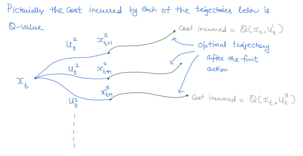
Thus, the optimal control can also be written as:

$$u_t^*(x_t) = \argmin_{u_t}Q(x_t, u_t)$$

Note that the optimal control is state-dependent, i.e., it is a feedback control.

Example: Discrete-time LQR

Please visit this page for more detailed information.

Inclusion of Control Bounds and Computation of Control

In dynamic programming, we can also easily include control bounds. Suppose $\underline{u} \leq u_t \leq \bar{u}$. In such a case, the Bellman equation can be re-written as:

$$V(x_t, t) = \min_{u_t\in [\underline{u}, \bar{u}]}\{\mathcal{L}\left(x_{t}, u_{t}\right)+V\left(x_{t+1}, t+1\right)\} \\ \text{ with } \; V(x, T+1) = l(x)$$

However, computation of the optimal control can be challenging even for simple systems. To see this, consider a simple case where $\alpha \equiv 0$ (i.e., there is no running cost) and $f_D(x, u)=f_1(x)+f_2(x) u$ (i.e., dynamics are control affine).

Recall,

$$\begin{aligned} u_t^* & =\argmin_{u_t} V\left(x_{t+1}, t+1\right) \\ & =\argmin_{u_t} V\left(f_1(x)+f_2(x) u_t, t+1\right) \end{aligned}$$

This is a complex optimization problem. For example, if $V$ is any non-linear function of $x$ (which is not atypical), the above is a non-convex problem and solving this problem can be quite challenging. This is one of the core reasons why DQN is primarily for discrete actions (where this optimization becomes easier) as actor-critic methods are used in RL. However, as we will see later, optimal control computation is a much easier problem in continuous time.

---

Continuous-time Optimal Control Problem

One of the advantages of dynamic programming is that it can be used to solve both discrete and continuous-time OC problems. In continuous time, the principle of optimality reads:

$$V(x, t)=\min _{u(\cdot)}\{\underbrace{\int_{s=t}^{t+\delta} L(x(s), u(s)) d s}_{\text{Cost from }[t, t+\delta]}+\underbrace{V(x(t+\delta), t+\delta)}_{\text{Optimal cost from }t+\delta\text { onwards}}\}$$

Taking $\delta$ to be very smalls we can re-write the above euqation as

$$V(x, t)=\min _u\{L(x, u) \delta+V(x(t+\delta), t+\delta)\}$$

Apply Taylor expansion:

$$\begin{aligned} V(x(t+\delta), t+\delta) & =V(x(t), t)+\frac{\partial V}{\partial x} \cdot(x(t+\delta)-x(t)) +\frac{\partial V}{\partial t} \cdot(t+\delta-t)+h.o.t. \\ & =V(x, t)+\frac{\partial V}{\partial x} \cdot f(x, u) \delta+\frac{\partial V}{\partial t} \cdot \delta \\ & \Rightarrow V\left(x, t\right)=\min _u\left\{L(x, u) \delta+V(x, t)+\frac{\partial V}{\partial x}\cdot f(x, u) \delta+\frac{\partial V}{\partial t} \delta\right\} \\ & V(x, t)=V(x, t)+\frac{\partial V}{\partial t} \delta+\min _u\left\{L(x, u) \delta+\frac{\partial V}{\partial x} \cdot f(x, u) \delta\right\} \\ & \Rightarrow \delta\left[\frac{\partial V}{\partial t}+\min _u\left\{L(x, u)+\frac{\partial V}{\partial x} \cdot f(x, u)\right\}\right]=0 \\ & \end{aligned}$$

This needs to hold for all $\delta>0$.

Hamilton-Jacobi Bellman PDE

$$\frac{\partial V}{\partial t}+\min _u\left\{L(x, u)+\frac{\partial V}{\partial x} \cdot f(x, u)\right\}=0 \\ V(x, T) = l(x) \leftarrow \text{Terminal condition}$$

• HJB-PDE is a terminal-time PDE.
• The continuous-time counterpart of the Bellman equation.
• $L(x, u)+\frac{\partial V}{\partial x} \cdot f(x, u)=H(x, u, V) \text { Also called Hamiltonian}$
• If there is only terminal cost (i.e., there is no running cost), the HJB PDE reduces to:
  $$\frac{\partial V}{\partial t}+\min _u\left\{\frac{\partial V}{\partial x} \cdot f(x, u)\right\}=0$$
  This will be the PDE that we will solve for safety problems as we will see later.

Obtaining Optimal Control from the Value Function

$$\begin{aligned} u^*(x, t)= & \argmin_u H(x, u, V, t) \\ & =\argmin _u\left\{\frac{\partial V(x, t)}{\partial x} \cdot f(x, u)+L(x, u)\right\} \end{aligned}$$

Once again, we have a feedback control policy.

In the presence of control bounds, we have:

$$u^*(x, t)=\argmin_{\underline{u} \leq u \leq \bar{u}}\left\{\frac{\partial V(x, t)}{\partial x} \cdot f\left(x, u\right)+L(x, u)\right\}$$

Let's go back to the issue of actually computing the optimal control from the value function. Once again, consider the case where $\mathcal{L} \equiv 0$ and $f(x, u)=f_1(x)+f_2(x) u$.

$$\begin{aligned} u^*(x, t) & =\argmin_u \left\{\frac{\partial V(x, t)}{\partial x} \cdot\left(f_1(x)+f_2(x) u\right)\right\} \\ & =\argmin_u \left\{\frac{\partial V(x, t)}{\partial x} \cdot f_1(x)+\left(\frac{\partial V(x, t)}{\partial x} \cdot f_2(x)\right) u\right\} \end{aligned}$$

This is a linear optimization in $u$ and can easily be solved in an analytical fashion. So one of the advantages of applying DP in continuous time is that it significantly simplifies the computation of optimal control.

This makes continuous-time dynamic programming a very promising tool for solving continuous control tasks. It is a different question that how important continuous control is over discrete control.

---

Methods to Compute Value Function - Discrete Time

In discrete time, we are interested in solving the Bellman equation:

$$V\left(x_t, t\right) =\min _{u_t}\left\{\mathcal{L}\left(x_{t,} u_t\right)+V\left(x_{t+1}, t+1\right)\right\} \\ V\left(x, T+1\right) =l(x)$$

Closed-form Computation of $V$ :

• Typically, solving $V$ in closed form is not possible. But under rare conditions, e.g. LQR problems, $V$ can be computed in closed form by recursively using the Bellman equation starting from the terminal time.

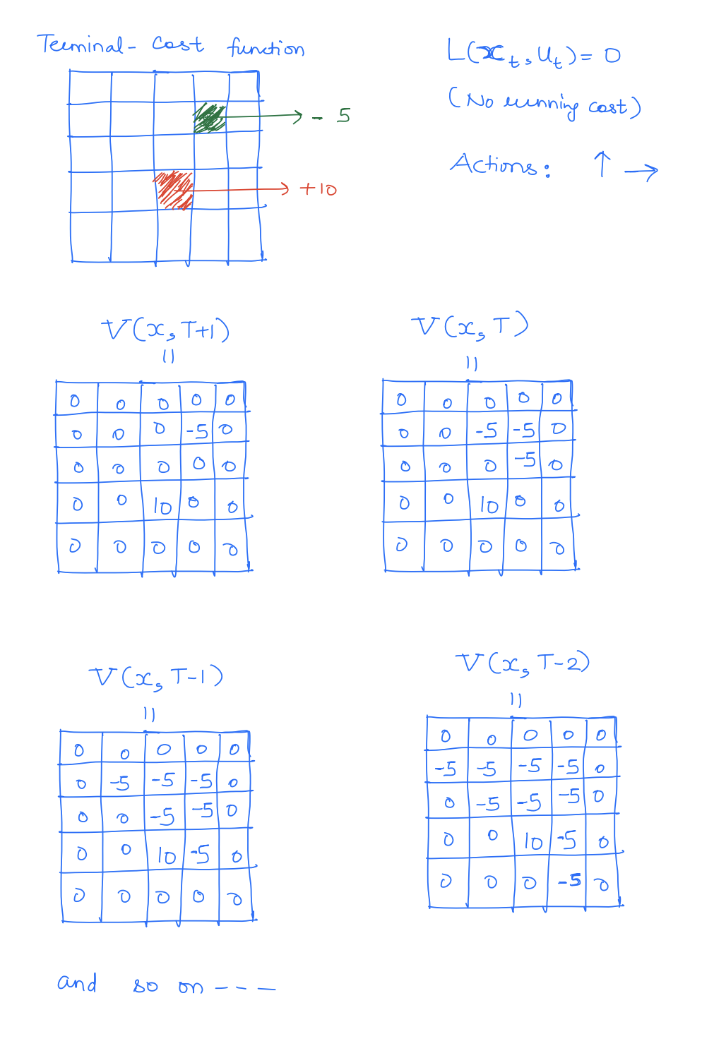
Tabular/Grid-based Methods to Compute $V$ :

• These methods discretize the states to create a grid in the state space, as well as discretize the control input.
• The value function is then computed over this grid starting from the terminal time.
• These methods suffer from the curse of dimensionality (the number of grid points scales exponentially in the number of states); thus, it is limited to low-dimensional systems.

Example: Grid-world

Function-approximator-based Methods:

• These methods try to approximate the value function through a parameterized function. That is,
  $$V(x, t) \equiv V\left(x, t ; \theta\right) \equiv V_\theta\left(x, t\right)$$
• The parameters are then computed to satisfy the Bellman equation as closely as possible. We want to find $\theta$ such that:
  $$\theta^*=\argmin_{\theta} \| V_\theta(x, t)-\min _u \left\{L(x, u)+V_\theta\left(x_{t+1}, t+1\right) \right\}\|+ \lambda\left\|V_\theta(x, T+1)-l(x)\right\|,$$
  i.e., satisfy the Bellman equation and the boundary condition.
• These function approximators include neural networks, quadratics/polynomials, linear combinations of predefined basis functions, etc. The most popular these days are neural networks.
• The above method is also called the fitted value iteration because we "fit" the value function that minimizes the Bellman error. When neural networks are used as the function approximator, the method is called neural fitted value iteration.
• There are several variants of the fitted value iteration algorithm to make them work well in practice. This includes learning the $Q$-function instead of the value function (DQN), learning policy and value function simultaneously (actor-critic methods), and so on.

---

Methods to Compute Value Function - Continuous Time

In continuous time, we are interested in solving the Hamilton-Jacobi Bellman PDE to obtain the value function:

$$\frac{\partial V}{\partial t}+\min _u\left\{L_C(x, u)+\frac{\partial V}{\partial x} \cdot f(x, u)\right\}=0 \\ V(x, T)=l(x)$$

Just like discrete time, we have three broad classes of methods to compute value function:

Closed-form Computation of $V$ :

• Can be done for a very restrictive class of OC problems
• Example: LQR problem

Mesh/Grid-based Methods

They solve this PDE using numerical integration over a grid of state and time. $\frac{\partial V}{\partial t}$ and $\frac{\partial V}{\partial x}$ are numerically approximated on the grid.

There are several toolboxes that you can download off the shelf for this:

• LST/helper OC
• BEACLS (c++)
• OptimizedDP (python)

These tools were primarily developed for reachability but they can easily handle any DP problem as well.

Similar to discrete time, these methods are limited to a fairly low-dimensional system (5D-6D systems max).

Function Approximation-based Methods

• Represent the value function as a parametrized function.
• A variety of function approximators are available including linear programs, quadratics, polynomials (SoS programming), zonotopes, and ellipsoids.
• Very recently, neural network-based function approximations have also been used (inspired by physics-informed neural networks). One such framework is DeepReach. DeepReach aims to solve the following problem:
  $$\theta^*=\argmin_{\theta}\left\|\frac{\partial V}{\partial t}+\min _u\left\{L(x, u)+\frac{\partial V}{\partial x}\cdot f(x, u)\right\}\right\|+\lambda\|V(x, T)-l(x)\|$$
  The value function is approximated as a neural network and $\theta$ is obtained by Stochastic Gradient Descent (SGD).
• These methods are able to compute value function only approximately though.