Model Predictive Control

MPC at its core is very similar in spirit to calculus of variations, in the sense that it solves the optimal control problem by leveraging concepts from optimization. However, it leverages the power of digital optimization and modern computers to solve this optimization problem. Thus, it is not surprising that the rise in popularity of MPC coincides with advances in computing and applied optimization.

Given this background, perhaps it is also not surprising that the MPC problem is often solved in discrete time (since continuous-time optimal control problem has an infinite number of optimization variables).

Mathematically

At time $t$, MPC solves the following optimization problem:

$$\begin{aligned} \min_{u_{t: T-1}} \quad & J\left(x_{t}, u_{t: T}, t\right) \\ \text{subject to} \quad & x_{s+1} =f_{D}\left(x_{s}, u_{s}\right) \\ & \underline{u} \leq u_{s} \leq \bar{u} \end{aligned}$$

• The optimization variables are $\left\{u_{t}, u_{t+1}\cdots u_{T-1}\right\}$ (explicit) and $\left\{x_{t+1},\cdots x_{T}\right\}$ (implicit). So the total number of variables are $(T-1-t) \times\left(n_{x}+n_{u}\right)$ where $n_{x}$ and $n_{u}$ are the dimensions of the state and control respectively.

• In general, the dynamics are non-linear and the cost is non-convex, making the above optimization problem non-convex. Modern MPC solvers often use a variety of methods to handle this non-convexity (e.g, sequential convex programming); however, more often than not, we can only expect to obtain a locally optimal solution.

Feedback control using MPC

Practical MPC approaches often solve the optimization problem above, apply the control input $u_{t}^{*}$ and then re-solve the optimization problem at time $t+1$. This provides a closed-loop, feedback controller for the autonomous system (as opposed to an open-loop controller obtained by solving the optimization problem only once). To understand this, Consider the following situation:

Suppose, you want to go from one corner of the room to another while following the red trajectory. Powered by the recent knowledge of optimal control, you set yourself an optimal control problem

$$\begin{aligned} \min_{u_{t: T}} \quad & \sum_{s=t}^{T}\left(p_{x}^{s}-g_{x}^{s}\right)^{2}+\left(p_{y}^{s}-g_{y}^{s}\right)^{2} \\ \text{subject to} \quad & \text{human dynamics} \\ & \text{step with length constraints} \end{aligned}$$

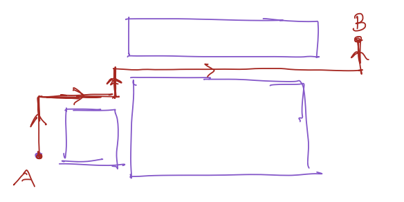
Your brain is really good at solving this optimal control problem and you came up with the following control commands to follow the red trajectory:

1. 4 steps forward
2. 5 steps right
3. 3 steps left
4. 10 steps right ... so on

Now, what do you think? With your eyes closed if you try to follow this path, would you be able to follow this exactly? Would you reach B? Not quite, sometimes we can but more often than not, we can't.

Now, suppose you get to walk with your eyes open. Would you be able to follow this path? Most likely so.

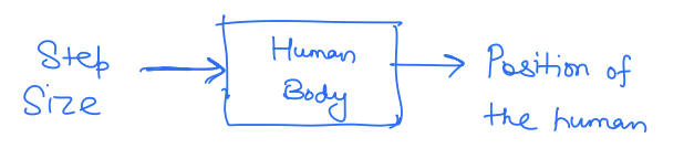
So why is that the case? Let's try to understand this from a control theory perspective. Here, the system is

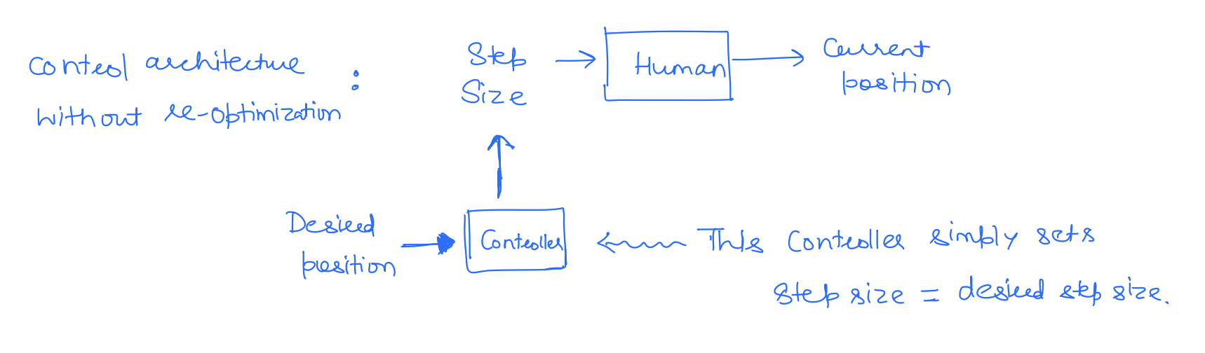
When we walk with our eyes closed, we are following a table of step commands, completely disregarding what our actual position (or output) is. These types of controllers are called open-loop controllers, where the input of the system does not depend on the output. The open-loop controllers completely ignore the fact that there is a reality gap between our model and our system, i.e., we have uncertainty in our system, so we won't quite end up where we think we would. Over time, these errors compound and we will end up in a completely different position.

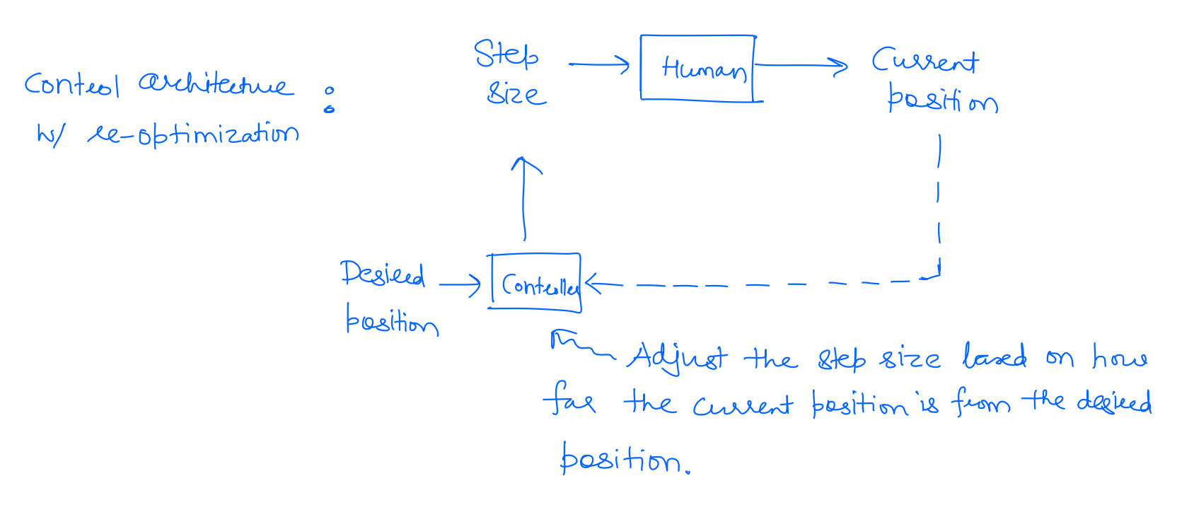
Whereas when you walk with open eyes, your next step corrects the errors you might make along the path. So for example, if I end up taking a big forward step, you might take only two more forward steps rather than 3. This adaptability of the input based on the output is called a closed-loop controller. This is precisely what we get by re-optimizing at the next time step in MPC -- depending on the actual next state of the robot, I get to adjust my control command to letter optimize my performance criterion.

Mathematically we solve a different optimization problem at each time step.

Time-step t

$$\begin{aligned} u_{t: T}^{*} = \argmin_{u_{t: T}} \quad &J\left(x_{t}, u_{t: T}, t\right) \\ \text{subject to} \quad & \text{dynamics} \\ & \text {constraints} \end{aligned}$$

Apply $u_t^*$ to the system, observe $x_{t+1}$

Time-step t+1

$$\begin{aligned} u_{t+1: T}^{*} = \argmin_{u_{t+1: T}} \quad &J\left(x_{t+1}, u_{t+1: T}, t+1\right) \\ \text{subject to} \quad & \text{dynamics} \\ & \text {constraints} \end{aligned}$$

Apply $u_{t+1}^*$ to the system, observe $x_{t+2}$

Receding Horizon MPC

One last practical detail to note about MPC is that it is often solved in a receding horizon fashion. Recall that the number of optimization variables scales linearly with the size of the time horizon over which the MPC problem is being solved. Since the number of optimization variables directly affects the time taken to solve the optimization problem, we often wanna keep the horizon to be small in order to be able to solve the problem fast enough, especially if we are doing it on resource-constrained systems.

Specifically, we solve the problem over the horizon $[t: t+H]$ at time $t$ s over the horizon $[t+1: t+H+1]$ at time $t+1$, and so on. Here, $H$ is typically far smaller than $T$.

Time-step t

$$\begin{aligned} u_{t: t+H}^{*} = \argmin_{u_{t: t+H}} \quad &J\left(x_{t}, u_{t: t+H}, t\right) \\ \text{subject to} \quad & \text{dynamics} \\ & \text {constraints} \end{aligned}$$

Apply $u_t^*$ to the system, observe $x_{t+1}$

Time-step t+1

$$\begin{aligned} u_{t+1: t+1+H}^{*} = \argmin_{u_{t+1: t+1+H}} \quad &J\left(x_{t+1}, u_{t+1: t+1+H}, t+1\right) \\ \text{subject to} \quad & \text{dynamics} \\ & \text {constraints} \end{aligned}$$

Apply $u_{t+1}^*$ to the system, observe $x_{t+2}$

A couple of things to note here: even though we will like the $H$ to be as small as possible (from a computational viewpoint), a too-small $H$ might lead to a greedy controller. On the other hand, a large $H$ might lead to a computationally intensive optimization problem. Selecting appropriate $H$ that balances off computation and optimality is often based on heuristics and is still an open problem in the MPC literature.

Summary

Pros	Cons
MPC can leverage modern compute to effectively solve complex optimal control problem.	Mostly effective in discrete-time.
Can handle non-linear dynamics, state constraints, and control bounds. (Key reason for its popularity in robotics	Often only solves the optimization problem locally; no guarantee of global solution.
Can account for behaviors that are optimal with respect to future.	The optimization parameters are often based on heuristic and can significantly affect the quality of the solution.
Can account for online changes in dynamics, cost function, constraints, etc.	Solution may not be recursively feasible.
	Can still be limiting for resource constrained robots.