More on Safety

---

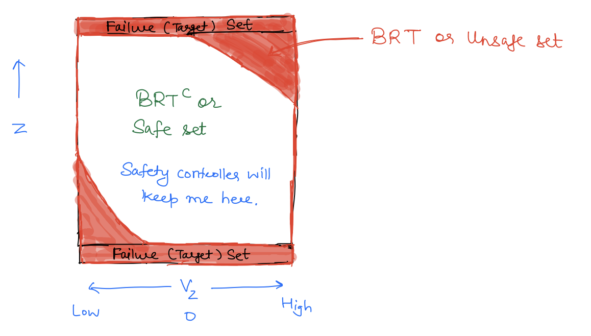
Safe Control

So far, we have seen how HJI-VI can be used to compute the $B R T(t)$ s i.e., the unsafe set of states. Conversely, if the system is outside the ${BRT}^{C}(t)$, then the HJI-VI also provides a safety-preserving controller. In this section, our focus is on studying that controller and how it can be used for safety filtering.

To derive a safety controller, let's go back to the discrete-time DP where the value function is defined by the Bellman equation:

$$V(x, t)=\max _{u}\left\{L(x, u)+V\left(x_{+}, t+1\right)\right\}$$

Here, the optimal controller at state $x$ at time $t$ is one that indeed achieves the above maximums i.e., the input that satisfies the principle of optimality:

$$u^{*}(x, t)=\argmax_{u}\left\{L(x, u)+V\left(x_{+}, t+1\right)\right\}$$

Indeed if I follow this optimal control sequence starting from state $x$ at time $t$, I will incur an overall optimal cost of $V(x, t)$.

In other words, $u^{*}\left(x, \cdot\right)$ is the control law that achieves the value $V(x, t)$.

Similarly, in continuous time, the Bellman equation is replaced by HJB PDE:

$$\frac{\partial V}{\partial t}+\max _{u}\left\{L(x, u)+\frac{\partial V}{\partial x} \cdot f(x, u)\right\}=0$$

Here also the optimal control $u^{*}\left(x, t\right)$ that actually achieves the value $V\left(x, t\right)$ is given by the one that satisfies the principle of optimality. In other words, it is the control that actually achieves the above maximum:

$$u^{*}(x, t)=\argmax_{u}\left\{L(x, u)+\frac{\partial V}{\partial x}(x, t) \cdot f(x, u)\right\}$$

The same principle applies in the context of reachability. If we are outside the unsafe set (ie. $V(x, t)>0$ ) and want to achieve this value over the time horizon $[t, T]$, we should apply the control input that satisfies the principle of optimality. Recall that HJI-VI is given as (in the absence of disturbance):

$$\begin{gathered} \min \left\{l(x)-V(x, t), \frac{\partial V}{\partial t}+\max _{u} \frac{\partial V}{\partial x} \cdot f(x, u)\right\}=0 \\ V(x, T)=l(x) \end{gathered}$$

The optimal control that the system can apply to maximize the signed distance to $\mathcal{L}$ is given by the controller that maximizes the Hamiltonian, i.e.,

$$u_{\text{safe}}^{*}(x, t)=\argmax_{u} \frac{\partial V(x, t)}{\partial x} \cdot f(x, u)$$

In the cases where the BRT converges, we can ignore the time argument. Letting $V^{*}(x)$ be the converged value function, the safety controller can be simplified as:

$$u_{\text{safe}}^{*}(x)=\argmax_u \frac{\partial V^{*}(x)}{\partial x} \cdot f(x, u)$$

• Intuitively, $u^{*}$ tries to align the dynamics of the system in the direction of increasing $V$, i.e., it pushes the system away from the unsafe set. In fact, applying $u_{\text{safe}}^{*}(x)$ at any state $x$ will take the system farthest possible from the unsafe set.

• If the system starts outside the BRT and applies $u_{\text{safe}}^{*}(x)$, it will remain outside the BRT.

• It is particularly easy to compute this safe control for control-affine systems dynamics. For such systems, the dynamics can be written as $f(x, u)=f_{1}(x)+f_{2}(x) u \leftarrow$ The dynamics are affine in control

  Thus,

  $$\frac{\partial V^{*}(x)}{\partial x} \cdot f(x, u)=\frac{\partial V^{*}}{\partial x} \cdot f_{1}(x)+\frac{\partial V^{*}}{\partial x} \cdot f_{2}(x) u$$
  $$u_{\text {safe }}^{*}(x)=\underset{u}{\operatorname{argmax}} \frac{\partial V^{*}}{\partial x} \cdot f_{1}(x)+\frac{\partial V^{*}}{\partial x} \cdot f_{2}(x) u=\underset{u}{\operatorname{argmax}} \frac{\partial V^{*}}{\partial x} \cdot f_{2}(x) u$$

  This is a linear objective function in $u$ and can easily be solved, allowing us to tractably compute the control law for control-affine systems.

Example: A Longitudinal Quadrotor

The system state is given as $x=\left[\begin{array}{l}z \\ v\end{array}\right]$ where $\quad \begin{aligned} & \dot{z}=v \\ & \dot{v}=k u+g\end{aligned}$.

Moreover let $|u| \leq \vec{u}$.

In this case, $f(x, u)=\left[\begin{array}{c}v \\ k u+g\end{array}\right] =\left[\begin{array}{l}v \\ g\end{array}\right]+\left[\begin{array}{l}0 \\ k\end{array}\right] u$

Thus, $u_{\text {safe}}^{*}=\argmax_u \frac{\partial v^{*}}{\partial x} \cdot f(x, u)$

Let $\frac{\partial V^{*}}{\partial x}=\left[\begin{array}{ll}p_{1}(x) & p_{2}(x)\end{array}\right] \Rightarrow \frac{\partial V^{*}}{\partial x} \cdot f(x, u)=\left[\begin{array}{ll}p_{1}(x) & p_{2}(x)\end{array}\right]\left(\left[\begin{array}{l}v \\ g\end{array}\right]+\left[\begin{array}{l}0 \\ k\end{array}\right]\right)$

$\frac{\partial v^{*}}{\partial x} \cdot f(x, u)=\left(p_{1}(x) v+p_{2}(x) g\right)+\left(p_{2}(x) k\right) u \leftarrow$ a linear function in $u$

$$\begin{aligned} u_{\text {safe}}^{*}(x)&=\argmax_{|u| \leqslant \bar{u}}\left(p_{1}(x) v+p_{2}(x) g\right)+\left(b_{2}(x) k\right) u \\ &=\left\{\begin{array}{c} \bar{u} \quad \text { if } \; p_{2}(x) \geqslant 0 \\ -\bar{u} \quad \text { if } \; p_{2}(x)<0 \end{array}\right. \end{aligned}$$

$\rightarrow$ A bang-bang safety control law (typical for control-affine systems)

Example: Planar Car

State: $\left[\begin{array}{l}p_{x} \\ b_{y} \\ \theta\end{array}\right]$ with dynamics: $f(x, u)=\left[\begin{array}{c}v \cos \theta \\ v \sin \theta \\ \omega\end{array}\right]$

System control: $\omega$ where $|\omega| \leqslant \bar{\omega}$

Once again, we have a control affine system

$$\begin{aligned} f(x, u)&=\left[\begin{array}{c} v \cos \theta \\ v \sin \theta \\ 0 \end{array}\right]+\left[\begin{array}{l} 0 \\ 0 \\ 1 \end{array}\right] u \\ u_{\text {safe }}^{*}&=\argmax_{u} \frac{\partial V^{*}}{\partial x} \cdot\left(f_{1}(x)+f_{2}(x) u\right) \\ & =\argmax_u \left[p_{1}(x) \quad p_{2}(x) \quad p_{3}(x)\right] f_{2}(x) u \\ & = \operatorname{agmax} p_{3}(x) u \\ & =\left\{\begin{array}{l} \bar{\omega} \quad \text { if } \; p_{3}(x) \geqslant 0 \\ -\bar{\omega} \quad \text { if } \; p_{3}(x)<0 \end{array}\right. \end{aligned}$$

Example: Non-control-affine

Sometimes even when the system is not control-affine we can compute the safety control law. For example, consider the following 2D human dynamics model:

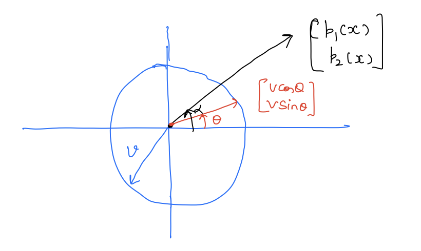
$$x=\left[\begin{array}{l} p_{x} \\ b_{y} \end{array}\right] \text { with } f(x, u)=\left[\begin{array}{l} v \cos \theta \\ v \sin \theta \end{array}\right]$$

Here, $u=\theta$ (the heading of the human). The system dynamics here are not linear or affine in $\theta$.

$$u_{\text {safe }}^{*}(x)=\argmax_u \left[\begin{array}{ll} p_{1}(x) & p_{2}(x) \end{array}\right]\left[\begin{array}{c} v \cos \theta \\ v \sin \theta \end{array}\right]$$

The above objective is a dot product between two vectors. Pictorially:

If we want to maximize the dot product, we should pick $\theta=\alpha$. Thus, $u_{\text {safe}}^{*}(x)=\alpha(x)$ where $\alpha(x)=\tan ^{-1}\left(\frac{p_{2}(x)}{p_{1}(x)}\right)$

---

Safety Filtering

Often in robotic systems, we not only care about safety but also care about achieving a performance objective. After all, a self-driving car is safe if it doesn't move at all, but such a case is hard of any use from a practical viewpoint. In such cases, it is important to maintain performance while ensuring safety. One way to do so is via safety filtering.

The idea of safety filtering is to continue to apply a nominal performance controller (computed via MPC, RL, or even PID controller) until the safety is at risk; otherwise, apply a safety controller.

Let $u_{\text{norm}}(x)$ be a nominal controller at state $x$. This controller might have been computed using MPC, RL or any other control mechanism. But $u_{\text{norm}}(x)$ may not be sufficient to ensure safety (e.g., when it doesn't take obstacles into account.) A control law that trade-off safety with performance is given by:

$$u^{*}(x)= \begin{cases}u_{\text {norm}}(x) & \text { if system is safe } \\ u_{\text {safe}}^{*}(x) & \text { if safety at risk }\end{cases}$$

But how do we know when safety is at risk? Well, we know the system is safe as long as it is outside the unsafe set. Thus,

$$u^{x}(x)= \begin{cases}u_{\text{norm}}(x) & \text { if } V^{x}(x)>0 \\ u_{\text {safe }}^{x}(x) & \text { if } V^{x}(x)=0 \end{cases} \tag{A}$$

The control law in A is called least-restrictive safety filtering because it minimally interferes with the performance controller and only overrides it when the system safety is at risk.

The problem with the control law in (A) is that it leads to a sudden switch in the control policy near the boundary of the unsafe set which might deviate significantly from the nominal controller. Moreover, it is sufficient to apply any safe controller and not necessarily the one that maximizes the value function. Thus, we can devise an alternative safety filtering lave as follows:

$$\left.\begin{array}{rl} u^{*}(x)=& \argmin_u\left\|u-u_{\text {norm}}\right\|_{2}^{2} \\ & \text { s.t. } u \text { is safe } \end{array}\right\} \begin{aligned} & \text {Remain as close to } \\ & u_{\text {norm}} \text{ as possible } \\ & \text {while maintaining safety } \end{aligned}$$

But how do we obtain the set of all safe controls?

$u$ is safe $\equiv V^{*}(x(t+\delta)) \geqslant 0$ where $\delta$ is the simulation timestep The above statement is saying that a control input $u$ is safe as long as the next state is still outside the BRT.

$$V^{*}(x(t+\delta)) \approx V^{*}(x)+\delta \frac{\partial V^{*}}{\partial x} \cdot f(x, u) \geq 0$$

$$\begin{aligned} \Rightarrow u^{*}(x)= & \argmin_u \left\|u-u_{\text {norm}}\right\|_{2}^{2} \\ & \text { s.t. } V^{*}(x)+\delta \frac{\partial V^{x}}{\partial x} \cdot f(x, u) \geqslant 0 \end{aligned}$$

For a control affine system:

$$f\left(x, u\right)=f_{1}(x)+f_{2}(x) u$$

Thus, the constraint can be re-written as:

$$V^{*}(x)+\delta \frac{\partial V^{*}}{\partial x} \cdot f_{1}(x)+\delta \frac{\partial V^{*}}{\partial x} \cdot f_{2}(x) u \geqslant 0$$

Since we know $x$ and we know $V^{*}$, the above constraint is a linear constraint in $u$. Let's write the above constraint generally as $A u+b \geqslant 0$ where

$$\begin{aligned} A&=\delta \frac{\partial V^{*}}{\partial x} \cdot f_{2}(x) \\ b&=V^{*}(x)+\delta \frac{\partial V^{*}}{\partial x} \cdot f_{1}(x) \end{aligned}$$

Thus, the safety filtering law can be written as:

$$\begin{aligned} u^{*}(x)=&\argmin_u \left\|u-u_{\text {norm}}\right\|_{2}^{2} \\ & \text { s.t. } A u+b \geqslant 0 \end{aligned} \tag{B}$$

The safety filtering law in (B) is a QP-based law and is quite popular in robotics. because it can be efficiently solved online.

• Note that people use a variety of cost functions, including $\|u\|^{2}$ for minimum energy control, $\left\|u-u_{\text {last}}\right\|_{2}^{2}$ for minimum jerk control etc.

Example: Longitudinal Quadrotor

$$\begin{aligned} & f(x)=\left[\begin{array}{l} v \\ g \end{array}\right]+\left[\begin{array}{l} 0 \\ k \end{array}\right] u \quad \text { and let } \frac{\partial v^{*}}{\partial x}(x)=\left[p_{1}(x) \quad p_{2}(x)\right] \text { as before. } \\ & A=\delta\left[p_{1}(x) \quad p_{2}(x)\right]\left[\begin{array}{l} 0 \\ k \end{array}\right] u=\delta p_{2}(x) k u \\ & b=V^{*}(x)+\delta p_{1}(x) v+\delta p_{2}(x) g \end{aligned}$$

QP problem that needs to be solved at $x$ is:

$$\begin{aligned} & \min _{u}\left\|u-u_{\text {norm}}\right\|^{2} \\ & \text { s.t. }\left(\delta p_{2}(x) k\right) u \leq\left(V^{*}(x)+\delta p_{1}(x) v+\delta p_{2}(x) g\right) \end{aligned}$$

Example: Planar Vehicle

$$\begin{aligned} f(x) & =\left[\begin{array}{c} v \cos \theta \\ v \sin \theta \\ \omega \end{array}\right]=\left[\begin{array}{c} v \cos \theta \\ v \sin \theta \\ 0 \end{array}\right]+\left[\begin{array}{l} 0 \\ 0 \\ 1 \end{array}\right] \omega \\ A & =\delta p_{3}(x) \\ b & =V^{*}(x)+\delta p_{1}(x) v \cos \theta+\delta p_{2}(x) v \sin \theta \end{aligned}$$

---

Bringing Back Disturbance

The above safety filtering mechanisms can also be applied in the presence of uncertainty. Let's first look at the least restrictive controller. There $u_{\text{safe}}^{*}(x)$ is now given as:

$$u_{\text {safe}}^{*}(x)=\argmax_{u} \min _{d} \frac{\partial V^{*}(x)}{\partial x} \cdot f(x, u, d)$$

A particularly interesting class of dynamics is control and disturbance affine dynamics:

$$f\left(x, u, d\right)=f_{1}(x)+f_{2}(x) u+f_{3}(x) d$$

Thus,

$$\begin{aligned} u_{\text {safe}}^{*}(x) & =\argmax_u \frac{\partial V^{*}(x)}{\partial x} \cdot f_{1}(x)+\frac{\partial V^{*}(x)}{\partial x} \cdot f_{2}(x) u +\min _{d} \frac{\partial V^{*}(x)}{\partial x} \cdot f_{3}(x) d \\ & =\argmax_u \frac{\partial V^{*}(x)}{\partial x} \cdot f_{2}(x) u \end{aligned}$$

Thus, the safety control does not directly depend on $d$, but indirectly it does because $V^{*}(x)$ and $\frac{\partial V^{*}}{\partial x}(x)$ depend on $d$.

Example

$$\begin{aligned} & \dot{z}=v \\ & \dot{v}=k u+g+d \end{aligned}$$

Let $-\bar{u} \leq u \leq \bar{u},-\bar{d} \leq d \leq \bar{d}$

Here, $x=\left[\begin{array}{l}z \\ v\end{array}\right]$. Also let $\frac{\partial V^{*}(x)}{\partial x}=\left[\begin{array}{l}p_{1}(x) \\ p_{2}(x)\end{array}\right]$

$$f_{1}(x)=\left[\begin{array}{l} v \\ g \end{array}\right] \quad f_{2}(x)=\left[\begin{array}{l} 0 \\ k \end{array}\right] \quad f_{3}(x)=\left[\begin{array}{l} 0 \\ 1 \end{array}\right]$$

$$\begin{aligned} u_{\text {safe}}^{*}(x)& =\argmax_u \min _{d}\left[\begin{array}{ll} p_{1}(x) & p_{2}(x) \end{array}\right]\left(\left[\begin{array}{l} v \\ g \end{array}\right]+\left[\begin{array}{l} 0 \\ k \end{array}\right] u+\left[\begin{array}{l} 0 \\ 1 \end{array}\right] d\right) \\ & =\argmax_u \left[\begin{array}{ll} p_{1}(x) & p_{2}(x) \end{array}\right]\left[\begin{array}{l} 0 \\ k \end{array}\right] u \\ & =\argmax_u \left(p_{2}(x) k\right) u \\ & = \begin{cases}\bar{u} & \text { if } \; p_2(x) \geqslant 0 \\ -\bar{u} & \text{ otherwise }\end{cases} \end{aligned}$$

• A similar analysis can be done for the planar vehicle.

QP-based Safety Filter

Now, let's move on to the QP-based safety filter. Once again we want to pick a control input among the set of safe controls that is closest to $u_{\text {norm}}$.

$$\begin{aligned} u^{x}(x)=&\arg \min \left\|u-u_{\text {norm}}\right\|_{2}^{2} \\ & \text{s.t. } u \text { is safe } \end{aligned}$$

$$\begin{array}{r} u \text { is safe } \equiv \min_d V^{*}(x(t+\delta)) \geqslant 0 \leftarrow \text { even under the worst-case } \\ \text { disturbance, the next state } \\ \text { is outside the BRT } \end{array}$$

$$\begin{aligned} V^{*}(x(t+\delta))&=V^{*}(x)+\delta \frac{\partial V^{*}}{\partial x} \cdot f\left(x, u, d\right) \\ & =V^{*}(x)+\delta \frac{\partial V^{*}}{\partial x} \cdot f_{1}(x)+\delta \frac{\partial V^{*}}{\partial x} \cdot f_{3}(x) d+\delta \frac{\partial V^{x}}{\partial x} f_{2}(x) u \\ \min_d V^{*}(x(t+\delta))&=\left(V^{*}(x)+\delta \frac{\partial V^{*}}{\partial x} \cdot f_{1}(x)\right)+\min _{d} \delta \frac{\partial V^{*}}{\partial x} \cdot f_{3}(x) d +\delta \frac{\partial V^{*}}{\partial x} \cdot f_{2}(x) u \\ & =\left(V^{*}(x)+\delta \frac{\partial V^{*}}{\partial x} \cdot f_{1}(x)\right)+\delta \frac{\partial V^{*}}{\partial x} \cdot f_{3}(x) d^{*}+\delta \frac{\partial V^{*}}{\partial x} \cdot f_{2}(x) u \end{aligned}$$

Where $d^*=\argmin_d \frac{\partial V^*}{\partial x} \cdot f_3(x) d$. Once again $d^*$ can be easily found for affine dynamical systems.

Again, we have a constraint of form $A u+b \geqslant 0$, resulting in a QP. It is just that we have an additional offset of $\delta \cdot \frac{\partial V^{*}}{\partial x} \cdot f_{3}(x) d^{*}$ in $b$.

Example: Quadrotor Again

$$\frac{\partial V^{*}(x)}{\partial x} \cdot f_{1}(x)=v p_{1}(x)+g p_{2}(x)$$

$$\begin{aligned} d^{*}&=\argmin_d \frac{\partial V^{*}(x)}{\partial x} \cdot f_{3}(x) d \\ & =\argmin _{d} p_{2}(x) d \\ & =\left\{\begin{array}{l} -\bar{d} \quad \text { if } \; p_{2}(x) \geqslant 0 \\ \bar{d} \quad \text { if } \; p_{2}(x)<0 \end{array}\right. \end{aligned}$$

Thus, $\frac{\partial V^{*}(x)}{\partial x} \cdot f_{3}(x) d^{*}=p_{2}(x) d^{*}= \begin{cases}-p_{2}(x) \bar{d} & \text { if } p_{2}(x) \geqslant 0 \\ p_{2}(x) \bar{d} & \text { if } p_{2}(x)<0\end{cases}=\left|p_{2}(x)\right| \bar{d}$

$$\frac{\partial V^{*}(x)}{\partial x} \cdot f_{2}(x)=p_{2}(x) k$$

Thus, the linear constraint is given by:

$$\begin{aligned} & b=V^{*}(x)+\delta V p_{1}(x)+\delta g p_{2}(x)+\delta\left|p_{2}(x)\right| \bar{d} \\ & A=\delta p_{2}(x) k \\ & A u+b \geqslant 0 \end{aligned}$$

Planar Vehicle Example

$$\begin{gathered} f(x, u, d)=\left[\begin{array}{c} v \cos \theta+d_x \\ v \sin \theta+d_y \\ \omega \end{array}\right] \quad \text { where }|\omega| \leq \bar{\omega} \leftarrow \text { control, } \left\| \begin{array}{c} d_{x} \\ d_y \end{array}\right\| \leq \bar{d} \leftarrow \text { Disturbance } \\ f(x, u, d)=\left[\begin{array}{c} v \cos \theta \\ v \sin \theta \\ 0 \end{array}\right]+\left[\begin{array}{l} 0 \\ 0 \\ 1 \end{array}\right] \omega+\left[\begin{array}{cc} 1 & 0 \\ 0 & 1 \\ 0 & 0 \end{array}\right]\left(\begin{array}{c} d x \\ d y \end{array}\right) \leftarrow \text { 2D disturbance } \end{gathered}$$

Safety Filtering Pros and Cons

Pros

A very practical way to ensure safety on top of any nominal and potentially unsafe policy, including learning-based policies.

Cons

Only greedily optimize for performance. Doesn't take future policy or performance into account. It can lead to suboptimal performance in the future.