State-Space Representation

---

The notion of the state of a dynamic system is a fundamental notion in physics. The basic premise of Newtonian dynamics is that the future evolution of a dynamic process is entirely determined by its present state, following this abstract definition:

The state of a dynamic system is a set of physical quantities, the specification of which (in the absence of external excitation) completely determines the evolution of the system.

Basics of Control Theory

System and control theory provides a set of powerful frameworks that allow us to specify complex system behaviors with simple mathematical functions. One such framework that is particularly conducive to describing robotic systems is state-space representation.

In the state space representation, the system has:

State

• $x(t) \in \mathbb{R}^{n}$ (often written compactly as $x$)

• State describes the characteristics of interest in a system.

• Ex: it could be the 2D positions speed, and orientation for a ground wheeled robot or the joint configuration for a manipulator.

Control/Action

• $u(t) \in \mathbb{R}^{m}$ inputs that we can choose at each instance in time

• Ex: Accelecation/deceleration and stewing for a ground robot or motor torques for a robot manipulator.

Output/Observation

• $y(t) \in \mathbb{R}^{L}$ outputs that are actually measurable (typically through some sensors) Ex: Speed through a speedometer, position through a GPS etc.

• For now, we will assume that $y=x$, but it is often not the case, especially for modern, perception-driven robotic systems.

System Dynamics

How the system state evolves over time.

Continuous-time	Discrete-time
$t \in \mathbb{R}$	$t \in \mathbb{Z}$
$\frac{d x(t)}{d t}=\dot{x}(t)=f(x(t), u(t))$	$x_{t+1}=f\left(x_{t,} u_{t}\right)$
More common in control theory and system theory.	More common in RL, robotics these days because of the ease of compute and optimization.

It is also common practice to obtain a discrete approximation of continuous-time dynamics:

$$x_{t+1}=x_{t}+\Delta T \cdot f(x, u) \leftarrow \text { Forward Euler discretization accurate for small $\triangle T$.}$$

Example: Longitudinal quadrotor motion

$$x=\left[\begin{array}{l} p_{z} \\ v_{z} \end{array}\right]$$

$$\dot{x}=\left[\begin{array}{l} \dot{p}_{z} \\ \dot{v}_{z} \end{array}\right]=\left[\begin{array}{c} v_{z} \\ k_T{u} + g + k_0 \\ \end{array}\right].$$

Trajectory Notation

Note that state and control are all functions of time. To make the time dependence explicit, we use the trajectory notation.

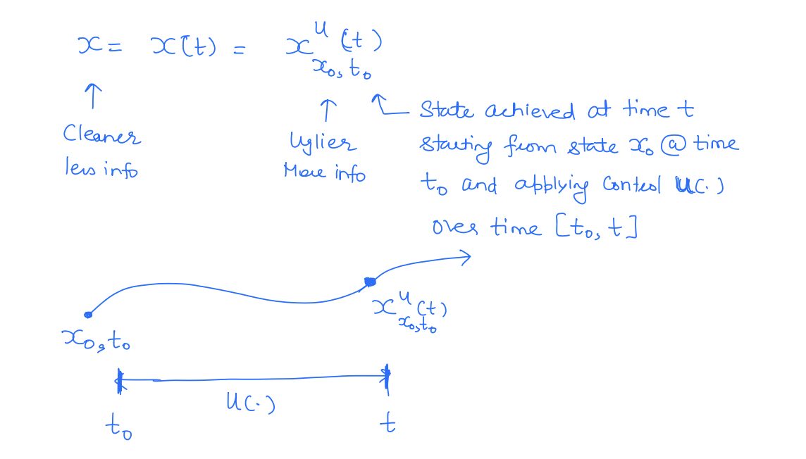
The trajectory over an entire time interval is also referred to as $x(\cdot)$. Similarly, the control function over the time interval is compactly written as $u(\cdot)$.

---

Need for Safety Analysis

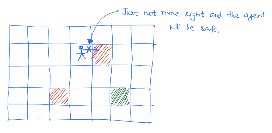
Before we move any further, let's briefly discuss why we even need to do a safety analysis. I mean if we know our failure set, isn't that enough? For instance, in machine learning, we often use a "grid-world" model of the world where the agent can move left, right, up, and down and we just need to avoid unsafe blocks. Why is the real world more complicated?

Reason 1: Inevitable Collision

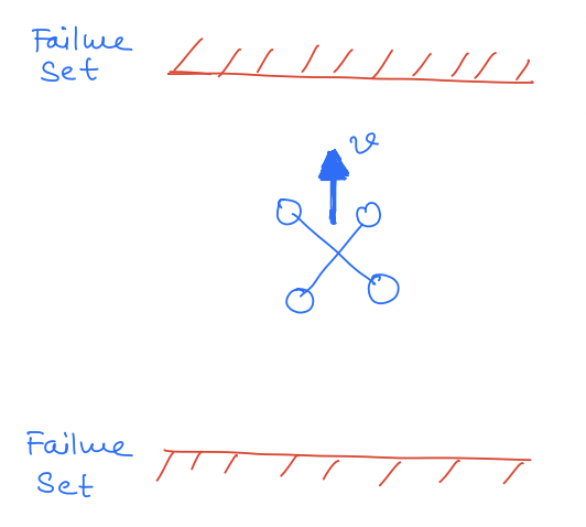
There may exist states from which you will reach the failure set even if you apply your optimal safe control.

For example, in this case, if the drone is moving at a very high speed toward the ceiling then it can't avoid a collision with the ceiling despite the best effort.

In fact, if we look at the unsafe set in this case, it looks as follows:

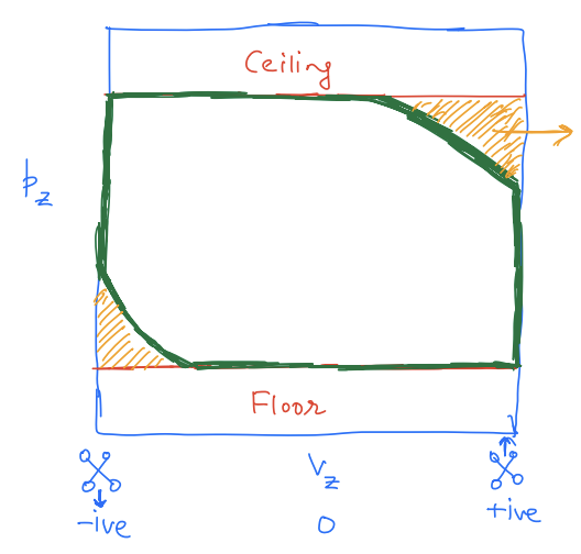
The yellow region is unsafe because the drone is too close to the ceiling and moving at a high speed toward it.

Reason 2: Uncertainty

Even though we represent the actual system with a mathematical model, a model will never be fully accurate and only partially represent the actual system.

All models are wrong (but some are useful).

— George Box

As an example, consider our longitudinal quadrotor model.

Our simple model

$$\begin{aligned} & x=\left[\begin{array}{l}p_{z} \\v_{z}\end{array}\right] \\ & \dot{p}_{z}=v_{z} \\ & \dot{v}_{z}=g+k_{T} u+k_{0} \\ & u: \text{Normalized thrust} \end{aligned}$$

Advanced model

$$\begin{aligned} & x=\left[\begin{array}{l}p_{z} \\v_{z} \\ \phi \\ w_x\end{array}\right] \\ & \dot{p}_{z}=v_{z} \\ & \dot{v}_{z}=g+k \cos{\phi} (F_1 + F_2) \\ & \dot{\phi} = w \\ & \dot{w}=k(F_1-F_2) \end{aligned}$$

The model is still not perfect though!

This tension b/w the sophistication of a model and the tractability of analysis is fundamental in robotics and control.

In other words, all models have a reality gap which we need to take into account during the safety analysis if we hope to ensure the safeness of the actual system. In fact, accounting for this uncertainty is so fundamental that I feel like this is often a key distinction between the capabilities of various safety analysis methods (as we will see later in this course). For now, let's dive deeper into various types of uncertainties that might be present in an autonomous system.

---

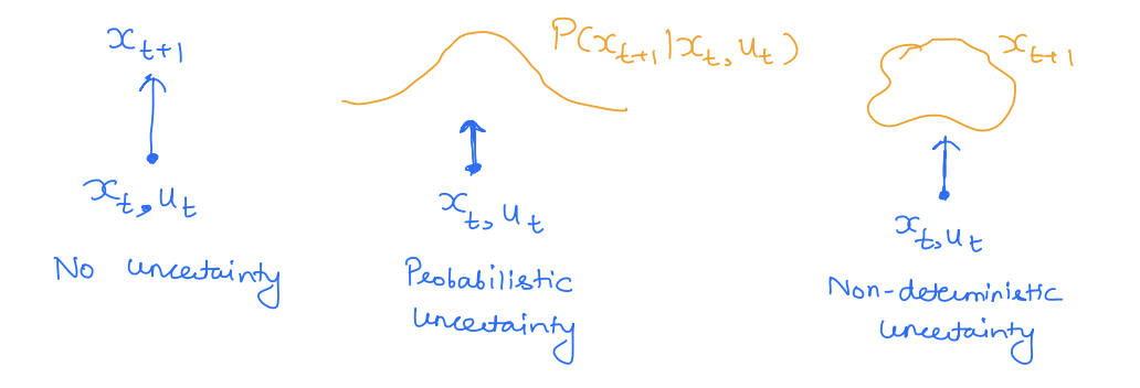
Uncertainty Representation

Uncertainty in a dynamic system can be classified by its nature and its representation. For example, uncertainty can be represented non-deterministically or probabilistically. Similarly, uncertainty can be structured or unstructured.

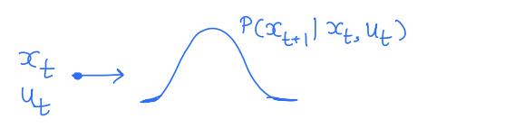
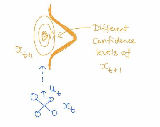
Probabilistic

• Uncertainty is modeled to have a distribution.

• In discrete time, we have:

  $$\begin{aligned} & x_{t+1}=f\left(x_{t}, u_{t}, d_{t}\right) \end{aligned}$$

  $d_t$ represents uncertainty that follows some distribution. Thus, $x_{t+1}$ is a random variable where $x_{t+1} \sim P\left(x_{t+1} \mid x_{t}, u_{t}\right)$.

• Similarly, continuous time dynamics can be written with probabilistic dynamics.

  $$\dot{x}(t)=f\left(x(t), u(t), d(t)\right)$$

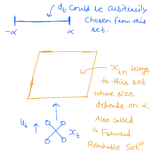
Non-deterministic

• The uncertainty belongs to a set, i.e. $d_{t} \in \varepsilon_{t} \leftarrow$ some set in $\mathbb{R}^{n}$.

• In discrete time, we have:

  $$\begin{aligned} & x_{t+1}=f\left(x_{t}, u_{t}, d_{t}\right) \\ & x_{t+1} \in F(x_t,u_t) \subseteq \mathbb{R}^{n} \\ & F: \text{some set (not a point)} \end{aligned}$$

  Thus, $x_{t+1}$ is a set of states and not a point in $\mathbb{R}^{n}$ anymore.

• Similarly, in continuous time

  $$\dot{x} \in F(x, u) \subseteq \mathbb{R}^{n}$$

Pictorially:

Example 2

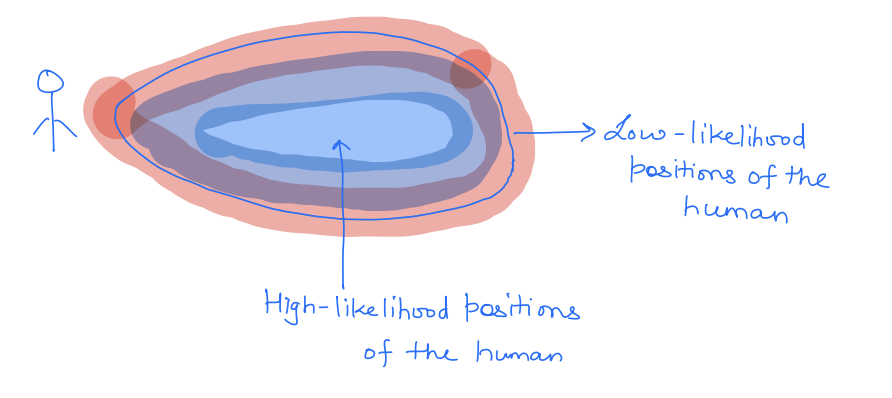
Suppose we are modeling a walking human. It is often modeled as a 2D particle moving in a 2D plane:

$$x=\left[\begin{array}{l} p_{x} \\ p_{y} \end{array}\right] \quad \begin{aligned} & \dot{p}_{x}=v \cos \theta \\ & \dot{p}_{y}=v \sin \theta \end{aligned}$$

These are the dynamics of a particle moving at a constant speed $v$. However, there is uncertainty in the direction of human motion (i.e., theta is uncertain and represents disturbance). In this case, a probabilistic uncertain model will assign different probabilities in different directions. Consequently, the future states of the human will look as follows:

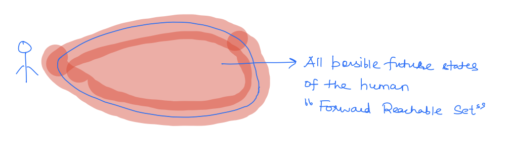
Whereas a non-deterministic uncertainty model will assume that $\theta$ belongs to some set and consequently will give a set of the possible future states of the human.

Cons

Probabilistic uncertainty	Non-deterministic uncertainty
Simple tractable distributions (e.g. Gaussian) often have unbounded support for the next state.	Sets can quickly g2ow in size resulting in a conservative plans, making open-loop plans intractable $\rightarrow$ will need closed-loop policies.
Distribution propagation through non-linear dynamics can be quite challenging.	Set propagation can be quite challenging $\rightarrow$ Level set methods.
Multimodality of $d_{t}$ or dynamics will lead to mixture models.

---

Types of Uncertainty

Uncertainty in a dynamic system can be classified as structured or unstructured uncertainty. In this section, we will study these two types of uncertainties.

Unstructured Uncertainty

Uncertainty is not characterized and modeled in an informed fashion. Typically, this type of uncertainty is used to account for unmodeled dynamics, high-frequency modes in the system, etc. Unstructured uncertainty models are often simpler to set up but are often made conservative.

A common choice is to model the uncertainty as an additive uncertainty, i.e.,

$$x_{t+1}=f_{D}\left(x_{t}, u_{t}\right)+d_{t}$$

As before, the uncertainty, $d_{t}$, can be represented probabilistically or non-deterministically.

Probabilistic

• $d_{t}$ - represented as a distribution

• $x_{t+1}$ in this case is a random variable.

Ex: In our quadrotor example, suppose that $d_{t} \sim N(0, \sigma)$

Non-deterministic

$d_{t}$ - often represented as a worst-case inclusion

$x_{t+1}$ in this care is a set and not a point.

Ex: $d_{t} \in[-\alpha, \alpha]$

Structured (Parametric) Uncertainty

Uncertainty enters dynamics in an "informed" manner, often as uncertain parameters. Compared to unstructured uncertainty, in structured uncertainty, we often know the "functional form" of uncertainty.

For example, consider our longitudinal quadrotor motion example. We might not know how exactly the motor torques are converted into the upward thrust of the quadrotor. In other words, we might have uncertainty in the $k_{T}$ parameter in the dynamics:

$$\begin{aligned} & \dot{p}_{z}=v_{z} \\ & \dot{v}_{z}=g+k_T u+k_{0} \end{aligned}$$

Summary

Probabilistic	Non-deterministic
Type of guarantees: probabilistic	Robust as "worst-case"
Optimize expected cost/performance	Worst case cost/performance
Probability bounds on failure	Failure impossibility conditions
Unstructured	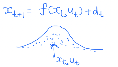Unstructured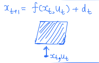
Structured	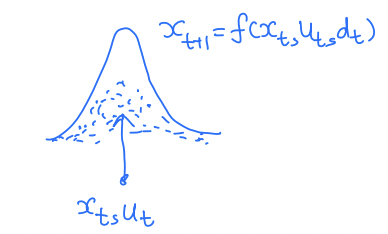Structured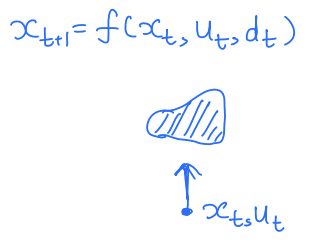

More peaked distribution / narrower sets when the uncertainty is structured.