Basic Distributional Quantities

---

Moments

Definition

The $k$ th raw moment of a random variable is the expected (average) value of the $k$ th power of the variable, provided that it exists. It is denoted by $E(X^k)$ or by $\mu_k'$. The first raw moment is called the mean of the random variable and is usually denoted by $\mu$.

• Raw moments for continuous variables:

  $$\mu'_k=E(X^k)=\int_{-\infty}^{\infty} x^kf(x)dx$$

• Raw moments for discrete variables:

  $$\mu'_k=E(X^k)=\sum_{x} x^kp(x)$$

  In particular, $\mu'_1=E(X)=\mu$

Definition

The $k$ th central moment of a random variable is the expected value of the $k$ th power of the deviation of the variable from its mean. It is denoted by $E[(X-\mu)^k]$ or by $\mu_k$. The second central moment is usually called the variance and denoted $\sigma^2$ or $Var(X)$,and its square root, $\sigma$, is called the standard deviation. The ratio of the standard deviation to the mean is called the coefficient of variation.

• Central moments:

  $$\mu_k=E[(x-\mu)^k]$$

  • Variance:

    $\mu_2=E[(x-\mu)^2]=\sigma ^2$

  • Skewness:

    $\gamma_1=\mu_3/\sigma^3$

  • Kurtosis:

    $\gamma_2=\mu_4/\sigma^4$

---

Excess Loss Variable/Residual Life

Definition

For a given value of $d$ with $\mathrm{Pr}(X>d)>0$, the excess loss variable is $y^p = X-d$, given that $X>d$. Its expected value,

$$e(d)=E(X-d|X>d)$$

is called the mean excess loss function. Other names for this expectation are mean residual life function and complete expectation of life.

To understand this equation, we first review the concept that:

$$\mathrm{Pr}(a<X<b|X>d)=\frac{\mathrm{Pr}(a<X<b)}{\mathrm{Pr}(X>d)}$$

Also, the conditional density of $X$ given $X>d$ is :

$$\frac{f(x)}{S(d)}, x>d$$

We also have the mean excess loss or mean residual life:

$$E[(X-d)^k|X>d]=\int_{d}^{\infty}(x-d)^k\frac{f(x)}{S(d)}dx=e_k(d)$$

Integration by parts:

$$\begin{aligned} E[(X-d)^k|X>d] & =-(x-d)^k\left.\frac{S(x)}{S(d)}\right|_{d}^{\infty}+\int_{d}^{\infty}k(x-d)^{k-1}\frac{S(x)}{S(d)}dx \\ & =0+\int_{d}^{\infty}k(x-d)^{k-1}\frac{S(x)}{S(d)}dx \end{aligned}$$

If $k = 1$, the mean excess loss or mean residual life is:

$$E(X-d|X>d)=\int_{d}^{\infty}\frac{S(x)}{S(d)}dx$$

If $d = 0$, assuming $S(0)=1$ we have:

$$E(X)=\int_{0}^{\infty}S(x)dx$$

---

Left Censored and Shifted Variable

The equation is

$$Y^L= \begin{equation} (X-d)_+ = \left\{ \begin{array}{lr} 0, & x \le d \\ X-d, & x>d \end{array} \right. \end{equation}$$

It is left censored because values below $d$ are not ignored but are set equal to zero. There is no standard name or symbol for the moments of this variable. For dollar events, the distinction between the excess loss variable and the left censored and shifted variable is one of per payment versus per loss. In the per-payment situation, the variable exists only when a payment is made. The per-loss variable takes on the value zero whenever a loss produces no payment. We can calculate the moments by:

$$\begin{aligned} E[(X-d)^k_+] &=\int_{d}^{\infty}(x-d)^kf(x)dx\\ &=\sum_{x_j>d} (x_j-d)^kp(x_j)\\ &=e_k(d)S(d) \end{aligned}$$

---

Limited Loss Variable

$$Y=\begin{equation} (X\wedge u) = \left\{ \begin{array}{lr} X, & X<u \\ u, & X\ge u \end{array} \right. \end{equation}$$

The expected value of the above function is called the limited expected value.

Definition

This variable could also be called the right censored variable. It is right censored because values above $u$ are set equal to $u$. An insurance phenomenon that relates to this variable is the existence of a policy limit that sets a maximum on the benefit to be paid. Note that $(X-d)_++(X\wedge d)=X$. That is, buying one insurance policy with a limit of $d$ and another with a deductible of $d$ is equivalent to buying full coverage.

Now we have

$$E[(X\wedge u)^k]=\int_{-\infty}^{u}x^kf(x)dx+u^k[1-F(u)]$$

We can derive another interesting formula as follows:

$$\begin{aligned} \mathrm{E}\left[(X \wedge u)^k\right]= & \int_{-\infty}^0 x^k f(x) d x+\int_0^u {x^k f(x) d x}+u^k[1-F(u)] \\ = & \left.x^k F(x)\right|_{-\infty} ^0-\int_{-\infty}^0 k x^{k-1} F(x) d x \\ & -\left.x^k S(x)\right|_0 ^u+\int_0^u k x^{k-1} S(x) d x+u^k S(u) \\ = & -\int_{-\infty}^0 k x^{k-1} F(x) d x+\int_0^u k x^{k-1} S(x) d x \end{aligned}$$

where the second line uses integration by parts. For $k=1$, we have

$$\mathrm{E}(X \wedge u)=-\int_{-\infty}^0 F(x) d x+\int_0^u S(x) d x$$

---

Tails of Distribution

Definition

The right tail of a distribution is the portion of the distribution corresponding to large values of the random variable. Understanding large possible loss values is important because these have the greatest effect on total losses. Random variables that tend to assign higher probabilities to larger values are said to be heavier tailed. Tail weight can be a relative concept (model A has a heavier tail than model B) or an absolute concept (distributions with a certain property are classified as heavy tailed). When choosing models, tail weight can help narrow the choices or can confirm a choice for a model.

We normally have four ways to classify if a random variable is heavy or light-tailed.

1. Moments

If $\mu'_k=\int_{0}^\infty x^kf(x) d x<\infty$ for all $k$, then the distribution is light-tailed. Otherwise, it is heavy-tailed.

Example：

For the gamma distribution, the raw moments are

$$\begin{aligned} \mu_k^{\prime} & =\int_0^{\infty} x^k \frac{x^{\alpha-1} e^{-x / \theta}}{\Gamma(\alpha) \theta^\alpha} d x \\ & =\int_0^{\infty}(y \theta)^k \frac{(y \theta)^{\alpha-1} e^{-y}}{\Gamma(\alpha) \theta^\alpha} \theta d y, \quad \text { making the substitution } y=x / \theta \\ & =\frac{\theta^k}{\Gamma(\alpha)} \Gamma(\alpha+k)<\infty \text { for all } k>0 . \end{aligned}$$

For the Pareto distribution, they are

$$\begin{aligned} \mu_k^{\prime} & =\int_0^{\infty} x^k \frac{\alpha \theta^\alpha}{(x+\theta)^{\alpha+1}} d x \\ & =\int_\theta^{\infty}(y-\theta)^k \frac{\alpha \theta^\alpha}{y^{\alpha+1}} d y, \quad \text { making the substitution } y=x+\theta \\ & =\alpha \theta^\alpha \int_\theta^{\infty} \sum_{j=0}^k\left(\begin{array}{l} k \\ j \end{array}\right) y^{j-\alpha-1}(-\theta)^{k-j} d y, \quad \text { for integer values of } k . \end{aligned}$$

The integral exists only if all of the exponents on $y$ in the sum are less than $-1$, that is, if $j-\alpha-1<-1$ for all $j$ or, equivalently, if $k<\alpha$. Therefore, only some moments exist.

By this classification, the Pareto distribution is said to have a heavy tail and the gamma distribution is said to have a light tail.

2. Limit Tail Behavior

Definition

A commonly used indication that one distribution has a heavier tail than another distribution with the same mean is that the ratio of the two survival functions should diverge to infinity (with the heavier-tailed distribution in the numerator) as the argument becomes large. Note that it is equivalent to examine the ratio of density functions.

Example：

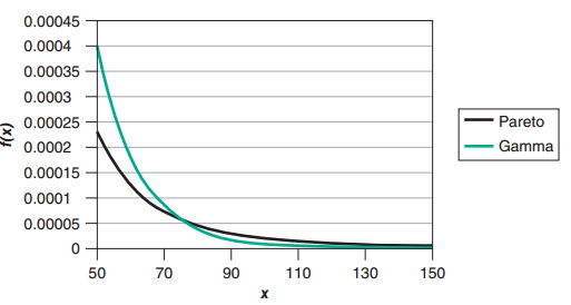
Demonstrate that the Pareto distribution has a heavier tail than the gamma distribution using the limit of the ratio of their density functions.

To avoid confusion, the letters $\tau$ and $\lambda$ will be used for the parameters of the gamma distribution instead of the customary $\alpha$ and $\theta$. Then, the required limit is

$$\begin{aligned} \lim _{x \rightarrow \infty} \frac{f_{\text {Pareto }}(x)}{f_{\text {gamma }}(x)} & =\lim_{x \rightarrow \infty} \frac{\alpha \theta^\alpha(x+\theta)^{-\alpha-1}}{x^{\tau-1} e^{-x / \lambda} \lambda^{-\tau} \Gamma(\tau)^{-1}} \\ & =c \lim _{x \rightarrow \infty} \frac{e^{x / \lambda}}{(x+\theta)^{\alpha+1} x^{\tau-1}} \\ & >c \lim_{x \rightarrow \infty} \frac{e^{x / \lambda}}{(x+\theta)^{\alpha+\tau}} \end{aligned}$$

and, either by application of L'Hôpital's rule or by remembering that exponentials go to infinity faster than polynomials, the limit is infinity. Figure below shows a portion of the density functions for a Pareto distribution with parameters $\alpha=3$ and $\theta=10$ and a gamma distribution with parameters $\alpha=\frac{1}{3}$ and $\theta=15$. Both distributions have a mean of 5 and a variance of 75 . The graph is consistent with the algebraic derivation.

3. Hazard Functions

Let's review the concept that $h(x)=\frac{f(x)}{S(x)}$, if the hazard function is increasing as x increases, then the random variable is light-tailed; if the hazard function is decreasing as x increases, the function is heavy-tailed. The hazard rate function for the Pareto distribution is

$$h(x)=\frac{f(x)}{S(x)}=\frac{\alpha \theta^\alpha(x+\theta)^{-\alpha-1}}{\theta^\alpha(x+\theta)^{-\alpha}}=\frac{\alpha}{x+\theta},$$

which is decreasing when fixing $\alpha$ and $\theta$. Therefore, the Pareto distribution is heavy-tailed.

4.Mean Excess Loss/Mean Residual Life

Definition

If the mean excess loss function is increasing in $d$, the distribution is considered to have a heavy tail. If the mean excess loss function is decreasing in $d$, the distribution is considered to have a light tail. The pattern is opposite to hazard function method.

Recap:

$e(d)=\frac{\int_d^{\infty}S(x)dx}{S(d)}$