Evaluating the Proportional Hazards Assumption

---

Background of Evaluating the PH Assumption

Recall from the previous note that the general form of the Cox PH model gives an expression for the hazard at time $t$ for an individual with a given specification of a set of explanatory variables denoted by the bold $\mathbf{X}$.

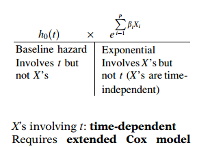
The Cox model formula says that the hazard at time $t$ is the product of two quantities. The first of these, $h_0(t)$, is called the baseline hazard function. The second quantity is the exponential expression $e$ to the linear sum of $\beta_iX_i$, where the sum is over the $p$ explanatory $X$ variables.

Cox PH model:

$$h(t,\mathbf{X})=h_0(t)e^{\sum_{i=1}^p\beta_iX_i}$$

where

$$\mathbf{X}=(X_1,X_2,...,X_p)$$

are explanatory/predictor variables

An important feature of this formula, which concerns the proportional hazards (PH) assumption, is that the baseline hazard is a function of t, but does not involve the $X$'s, whereas the exponential expression involves the $X$'s, but does not involve t. The $X$'s here are called time-independent $X$'s.

It is possible, nevertheless, to consider $X$'s that do involve t. Such $X$'s are called time-dependent variables. If time-dependent variables are considered, the Cox model form may still be used, but such a model no longer satisfies the PH assumption, and is called the extended Cox model, which we will discuss later.

From the Cox PH model, we can obtain a general formula, shown here, for estimating a hazard ratio that compares two specifications of the $X$'s. defined as $\mathbf{X}^*$ and $\mathbf{X}$.

Hazard ratio formula:

$$\hat{HR}=e^{\sum_{i=1}^p\hat{\beta_i}(\mathbf{X_i}^*-\mathbf{X_i})}$$

where $\mathbf{X}^*=(X^*_1,X^*_2,...,X^*_p)$

and $\mathbf{X}=(X_1,X_2,...,X_p)$

We can also obtain from the Cox model an expression for an adjusted survival curve. Here we show a general formula for obtaining adjusted survival curves comparing two groups adjusted for other variables in the model. Below this, we give a formula for a single adjusted survival curve that adjusts for all $X$'s in the model. Computer packages for these formulae use the mean value of each $X$ being adjusted in the computation of the adjusted curve.

The Cox PH model assumes that the hazard ratio comparing any two specifications of predictors is constant over time. Equivalently, this means that the hazard for one individual is proportional to the hazard for any other individual, where the proportionality constant is independent of time.

Adjusted survival curves comparing $E$ groups:

$$\hat{S}(t, \mathbf{X})=\left[\hat{S}_0(t)\right]^{\exp \left[\beta_1 E+\sum_{i \neq 1} \beta_i \bar{X}_i\right]}$$

Single curve:

$$S(t, \overline{\mathbf{X}})=\left[\hat{S}_0(t)\right]^{\exp \left[\sum_{i=1}^p \hat{\beta}_i \bar{X}_i\right]}$$

PH assumption: $\frac{\hat{h}\left(t, \mathbf{X}^*\right)}{\hat{h}(t, \mathbf{X})}=\hat{\theta}$, constant over $t$ i.e., $\hat{h}\left(t, \mathbf{X}^*\right)=\hat{\theta} \hat{h}(t, \mathbf{X})$

The PH assumption is not met if the graph of the hazards cross for two or more categories of a predictor of interest. However, even if the hazard functions do not cross, it is possible that the PH assumption is not met. Thus, rather than checking for crossing hazards, we must use other approaches to evaluate the reasonableness of the PH assumption.

Hazards cross: $\Rightarrow$ PH not met

Hazards don't cross $\nRightarrow$ PH met

---

Checking the Proportional Hazards Assumption: Overview

There are three general approaches for assesssing the PH assumption:

1. graphical
2. goodness-of-fit test
3. time-dependent variables

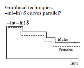
Graphical techniques:

There are two types of graphical techniques available. The most popular of these involves comparing estimated -ln(-ln) survivor curves over different (combinations of) categories of variables being investigated. We will describe such curves in detail in the next section. Parallel curves, say comparing males with females, indicate that the PH assumption is satisfied, as shown in this illustration for the variable Sex.

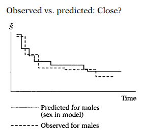
An alternative graphical approach is to compare observed with predicted survivor curves. The observed curves are derived for categories of the variable being assessed, say, Sex, without putting this variable in a PH model. The predicted curves are derived with this variable included in a PH model. If observed and predicted curves are close, then the PH assumption is reasonable.

Goodness-of-fit (GOF) tests

A second approach for assessing the PH assumption involves goodness-of-fit (GOF) tests. This approach provides large sample Z or chi-square statistics which can be computed for each variable in the model, adjusted for the other variables in the model. A p-value derived from a standard normal statistic is also given for each variable. This p-value is used for evaluating the PH assumption for that variable. A nonsignificant (i.e., large) p-value, say greater than 0.10, suggests that the PH assumption is reasonable, whereas a small p-value, say less than 0.05, suggests that the variable being tested does not satisfy this assumption.

Goodness-of-fit tests:

• Large sample Z or chi-square statistics

• Gives p-value for evaluating PH assumption for each variable in the model

p-value large $\Rightarrow$ PH satisfied (e.g. P $>0.10$)

p-value small $\Rightarrow$ PH not satisfied (e.g. P $<0.05$)

Time-dependent covariates

Definition

Extended Cox model: Add product term involving some function of time.

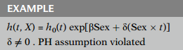
When time-dependent variables are used to assess the PH assumption for a time-independent variable, the Cox model is extended to contain product (i.e., interaction) terms involving the time-independent variable being assessed and some function of time.

For example, if the PH assumption is being assessed for Sex, a Cox model might be extended to include the variable "$\text{Sex} \times t$" in addition to Sex. If the coefficient of the product term turns out to be significant, we can conclude that the PH assumption is violated for Sex.

The GOF approach provides a single test statistic for each variable being assessed. This approach is not as subjective as the graphical approach nor as cumbersome computationally as the time-dependent variable approach. Nevertheless, a GOF test may be too "global" in that it may not detect specific departures from the PH assumption that may be observed from the other two approaches.