Intro to Survival Analysis

---

What is Survival Analysis

Definition

Survival analysis is defined as a collection of statistical procedures for data analysis for which the outcome variable of interests is time until an event occurs.

The time we referred to can be years, months, weeks, or days from the beginning of follow-up of an individual until an event occurs.

Alternatively, time can refer to the age of an individual when an event occurs. We typically refer to the time as survival time.

The event we referred to can be death, disease incidence, relapse from remission, recovery or any designated experience of interest that may happen to an individual. We typically refer to the event as a failure, because event of interest usually is negative individual experience.

Examples of Survival Analysis Problems

1. Leukemia patients/time in remission (weeks)
2. Disease-free cohort/time until heart disease (years)
3. Elderly (60+) population/time until death (years)
4. Parolees (recidivism study)/time until rearrest (weeks)
5. Heart transplants/time until death (months)

---

Censored Data

Definition

Censoring occurs when we have some information about individual survival time, but we don't know the survival time exactly.

Three Reasons Why Censoring May Occur

1. A person does not experience the event before the study ends
2. A person is lost to follow-up during the study period
3. A person withdraws from the study because of death (if death is not the event of interest) or some other reason (e.g., adverse drug reaction or other competing risk)

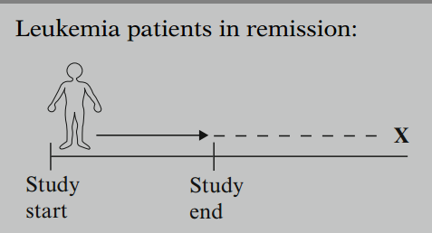
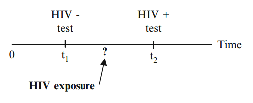
Example1

Consider leukemia patients followed until they go out of remission, shown here as $X$. If for a given patient, the study ends while the patient is still in remission (i.e., no event happened yet), then that patient's survival time is considered censored. We know that, for this person, the survival time is at least as long as the period that the person has been followed, but if the person goes out of remission after the study ends, we do not know the complete survival time.

Example2

Here is the graph that represents all of the three possible reasons why censoring may occur. An $X$ denotes a person who got the event:

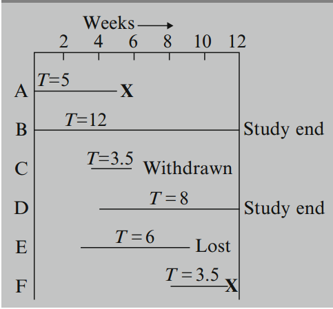
Person A is followed from the start of the study until getting the event at week 5; his survival time is 5 weeks and is not censored.

Peson B is observed from the start of the study but is followed to the end of the 12-week study period without getting the event; the survival time here is censored because we can say only that it is at least 12 weeks.

Person C enters the study between the week 2 and 3 and is followed until he withdraws from the study at the week 6; this person's survival time is censored after 3.5 weeks.

Person D enters at week 4 and is followed for the remainder of the study without getting the event; this person's censored time is 8 weeks.

Person E enters the study at week 3 and is followed until week 9, when he is lost to follow-up; his censored time is 6 weeks.

Person F enters at week 8 and is followed until getting the event at week 11.5. As with person A, there is no censoring here; the survival time is 3.5 weeks.

In summary, two patients (A and F) got the event, and four patients (B, C, D, and E) were censored.

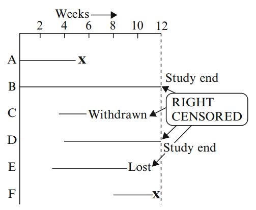
Different Types of Censoring

1. Right-censored: true survival time is equal to or greater than observed survival time.

   

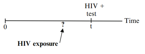
2. Left-censored: true survival time is less than or equal to the observed survival time

   

3. Interval-censored: true survival time is within a known time interval

   

Terminology and Notation

Time to event (survival time): $T$

Failure indicator:

$$d=\begin{equation} \left\{ \begin{array}{lr} 1, & event/failure \\ 0, & censored \end{array} \right. \end{equation}$$

---

Weibull Distribution

The probability density function is

$$f(x ; \theta, \tau)=\frac{\tau}{\theta} (\frac{x}{\theta})^{\tau-1} e^{(-x/\theta) ^\tau}$$

The cumulative distribution function is

$$F(x ; \theta, \tau)=1-e^{-(x/\theta)^\tau}$$

The hazard function is

$$h(x ; \theta, \tau)= \frac{\tau}{\theta}(\frac{x}{\theta})^{\tau-1}$$

The survial function is

$$S(x ; \theta, \tau)=e^{-(x/\theta)^\tau}$$

The hazard function is increasing if $\tau>1$. The hazard is decreasing if $\tau<1$.

---

Basic Data Layout for Understanding Analysis

In order to do analysis, we normally use the following data layout:

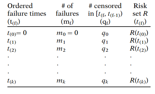
The first column in this table gives ordered failure times. These are denoted by $t's$ with subscripts within parentheses, starting with $t_{(0)}$, then $t_{(1)}$ and so on, up to $t_{(k)}$. Note that the parentheses surrounding the subscripts distinguish ordered failure times from the survival times previously given in the computer layout.

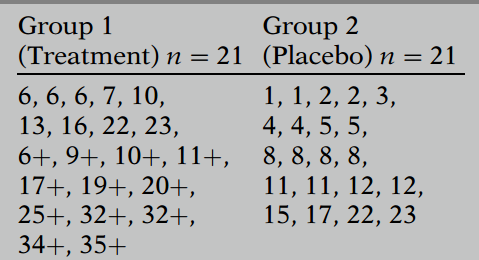
Now lets take a look at two experimental groups:

The first column in this table gives ordered failure times.

For example, using the remission data for group 1, we find that 9 of the 21 persons failed, including 3 persons at 6 weeks and 1 person each at 7, 10, 13, 16, 22, and 23 weeks. These nine failures have $k=7$ distinct survival times, because three persons had survival time 6 and we only count one of these 6's as distinct. The first ordered failure time for this group, denoted as $t_{(1)}$, is 6; the second ordered failure time $t_{(2)}$, is 7, and so on up to the seventh ordered failure time of 23.

The second column in the data layout gives frequency counts, denoted by $m_f$, of those persons who failed at each distinct failure time. When there are no ties at a certain failure time, then $m_f=1$.

The third column gives frequency counts, denoted by $q_f$, of those persons censored in the time interval starting with failure time $t_{(f)}$ up to the next failure time denoted $t_{(f+1)}$.

The last column in the table gives the "risk set." The risk set is not a numerical value or count but rather a collection of individuals. By definition, the risk set $R(t_{(f)})$ is the collection of individuals who have survived at least to time $t_{(f)}$; that is, each person in $R(t_{(f)})$ has a survival time that is $t_{(f)}$ or longer, regardless of whether the person has failed or is censored.

---

Descriptive Measures of Survival Experience

Let's still take a look at this table:

1. Ignoring the plus signs denoting censorship and average all 21 survival times for each group, we get an average, denoted by $\bar{T}$, of 17.1 weeks survival for the treatment group and 8.6 weeks for the placebo group.

2. We can also define average hazard rate, denoted as $\bar h$. This rate is defined by dividing the total number of failures by the sum of the observed survival times. In our example, $\bar h$ for group 1 is 9/359, and $\bar h$ for group 2 is 21/182. The higher the average hazard rate, the lower is the group's probability of surviving.

---

Censoring Assumptions

Definition

Independent Censoring means that within any subgroup of interest, the subjects who are censored at time $t$ should be representative of all the subjects in that subgroup who remained at risk at time $t$ with respect to their survival experience. In other words, censoring is independent provided that it is random within any subgroup of interest.

Comparing with independent censoring, random censoring is more restrictive.

Definition

Random Censoring means that subjects who are censored at time $t$ should be representative of all the study subjects who remained at risk at time $t$ with respect to their survival experience. In other words, the failure rate for subjects who are censored is assumed to be equal to the failure rate for subjects who remained in the risk set who are not censored.