Kaplan Meier Survival Curves Cont

---

The Log-Rank Test for Two Groups

When we state that two KM curves are "statistically equivalent," we mean that, based on a testing procedure that compares the two curves in some "overall sense," we do not have evidence to indicate that the true (population) survival curves are different.

In order to evaluate whether or not KM curves for two or more groups are statistically equivalent we use the most popular testing method called the log-rank test.

Definition

The log-rank test is a large-sample chi-square test that uses as its test criterion a statistic that provides an overall comparison of the KM curves being compared. This (log-rank) statistic, like many other statistics used in other kinds of chi-square tests, makes use of observed versus expected cell counts over categories of outcomes. The categories for the log-rank statistic are defined by each of the ordered failure times for the entire set of data being analyzed.

Example

Consider the comparison of the treatment (group 1) and placebo (group 2) subjects in the remission data on 42 leukemia patients. Let's take a look at the following table:

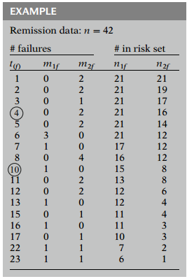
Here, for each ordered failure time, $t_{(f)}$, in the entire set of data, we show the numbers of subjects $(m_{if})$ failing at that time, separately by group ($i$), followed by the numbers of subjects $(n_{if})$ in the risk set at that time, also separately by group.

Thus, for example, at week 4, no subjects failed in group 1, whereas two subjects failed in group 2. Also, at week 4, the risk set for group 1 contains 21 persons, whereas the risk set for group 2 contains 16 persons.

Similarly, at week 10, 1 subject failed in group 1, and no subjects failed at group 2; the risk sets for each group contain 15 and 8 subjects, respectively.

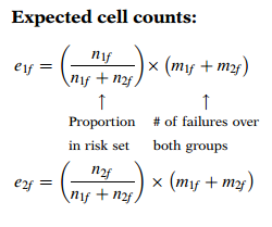
We now expand the previous table to include expected cell counts and observed minus expected values for each group at each ordered failure time. The formula for the expected cell counts is shown here for each group. For group 1, this formula computes the expected number at time $f$ (i.e., $e_{1f}$) as the proportion of the total subjects in both groups who are at risk at time $f$, that is, $n_{1f} /(n_{1f} + n_{2f})$, multiplied by the total number of failures at that time for both groups (i.e., $m_{1f} + m_{2f}$). For group 2, $e_{2f}$ is computed similarly.

In general, we have:

We have the new table:

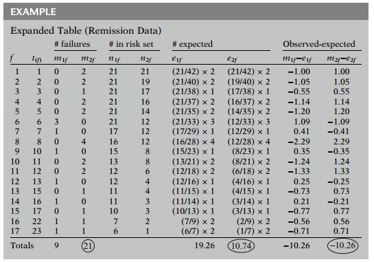
When two groups are being compared, the log-rank test statistic is formed using the sum of the observed minus expected counts over all failure times for one of the two groups. In this example, this sum is $-10.26$ for group 1 and $10.26$ for group 2. We will use the group 2 value to carry out the test, but as we can see, except for the minus sign, the difference is the same for the two groups.

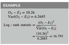
For the two-group case, the log-rank statistic, shown below, is computed by dividing the square of the summed observed minus expected score for one of the groups - say, group 2 - by the variance of the summed observed minus expected score.

Log-rank statistic =

$$\frac{(O_2-E_2)^2}{\mathrm{Var}(O_2-E_2)}$$

The expression for the estimated variance is shown here. For two groups, the variance formula is the same for each group. This variance formula involves the number in the risk set in each group ($n_{if}$) and the number of failures in each group ($m_{if}$) at time $f$. The summation is over all distinct failure times.

$$\mathrm{Var}(O_i-E_i)=\sum_{j}\frac{n_{1f}n_{2f}(m_{1f}+m_{2f})(n_{1f}+n_{2f}-m_{1f}-m_{2f})}{(n_{1f}+n_{2f})^2((n_{1f}+n_{2f}-1)}$$

where $i = 1, 2$

The null hypothesis being tested is that there is no overall difference between the two survival curves. Under this null hypothesis, the log-rank statistic is approximately chi-square with one degree of freedom. Thus, a P-value for the log-rank test is determined from tables of the chi-square distribution.

$$H_0: \text{no difference between survival curves}$$

Log-rank statistic ~$\chi^2$ with 1 df under $H_0$

Although the use of a computer is the easiest way to calculate the log-rank statistic, we can still calculate it by hand. We have already seen from earlier computations that the value of $O_2-E_2$ is $10.26$. The estimated variance of $O_2 -E_2$ is computed from the variance formula above to be $6.2685$. The log-rank statistic then is obtained by squaring $10.26$ and dividing by $6.285$, which yields $16.793$.

An approximation to the log-rank statistic, shown here, can be calculated using observed and expected values for each group without having to compute the variance formula. The approximate formula is of the classic chi-square form that sums over each group being compared the square of the observed minus expected value divided by the expected value

The approximate formula is:

$$X^2\approx\sum_{i}^{\text{number of groups}}\frac{(O_i-E_i)^2}{E_i}$$

The calculation of the approximate formula is shown here for the remission data. The expected values are $19.26$ and $10.74$ for groups 1 and 2, respectively. The chi-square value obtained is 15.276, which is slightly smaller than the log-rank statistic of $16.793$.

$$X^2 = \frac{(-10.26)^2}{19.26}+\frac{(10.26)^2}{10.74}=15.276$$

---

The Log-Rank Test for Several Groups

The log-rank test can also be used to compare three or more survival curves. The null hypothesis for this more general situation is that all survival curves are the same.

$$H_0 = \text{All survival curves are the same}$$

Log-rank statistics for > 2 groups involves variances and covariances of $O_i-E_i$.

In such case, we can use computer to do the computation. Therefore, we will not go into too much detials here. But, one thing we need to notice is, for $G(\ge 2)$ groups, the log-rank statistic ~ $\chi^2$ with $G-1$ df.

---

Confidence Intervals for KM Curves

We now describe how to calculate 95% confidence intervals (CIs) for the estimated Kaplan-Meier (KM) curve. The 95% CI formula for estimated KM probability at any time point over follow-up has the general large sample form shown below, where $\hat{S}_{KM}(t)$ denotes the KM survival estimate at time $t$ and $\mathrm{Var}[\hat{S}_{KM}(t)]$ denotes variance of $\hat{S}_{KM}(t)$. The most common approach used to calculate this variance uses the Greenwood's formula, also shown below.

95% CI for the KM curve:

$$\hat{S}_{KM}(t)\pm1.95\sqrt{\hat{\mathrm{Var}}[\hat{S}_{KM}(t)]}$$

Where Greenwood's formula for $\hat{\mathrm{Var}}[\hat{S}_{KM}(t)]$ is given by:

$$\hat{\mathrm{Var}}[\hat{S}_{KM}(t)]=(\hat{S}_{KM}(t))^2\sum_{f:t_{(t)}\le t}\frac{m_f}{n_f(n_f-m_f)}$$

$t_{(f)}=$ $f$-ordered failure time

$m_f=$ number of failures at $t_{(f)}$

$n_f=$ number in the risk set at $t_{(f)}$

The summation component of Greenwood's formula essentially gives at each failure time $t_{(f)}$, a weighted (by $1/n_f$) average of the conditional risk of failing at those failure times prior to $t_{(f)}$. Thus, the variance formula gives the square of the KM coordinate at each event time weighted by the cumulative estimate of the risk at time $t$.

We illustrate how Greenwood's variance is calculated for the treatment group (Group 1) of the remission times data described earlier. The layout for this computation is shown below.

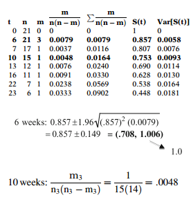
At 6 weeks, the estimate of the survival function is $0.857$. There were three events at 6 weeks and 21 patients at risk. Therefore, $m_f/n_f(n_f - m_f)=3/(21 \times 18) = 0.0079$. As this is the only component of the sum, the variance is then $0.0079 \times 0.8572 = 0.0058$. The corresponding 95% confidence interval is shown below, where the upper level should be modified to 1.

At 10 weeks, the estimate of the survival function is $0.753$. There was 1 event at 10 months and 15 patients at risk. Therefore, $m_f/n_f(n_f - m_f)= 1/ (15\times14) = 0.0048$.

$$\sum_{f:t_{(t)}\le t=10}\frac{m_f}{n_f(n_f-m_f)}=0.0079+0.0037+0.0048=0.0164$$

$$\hat{\mathrm{Var}}[\hat{S}_{KM}(t)]=(0.753)^2(0.0164)=0.0093$$

95% CI: $0.753\pm 1.96\sqrt{0.0093}=(0.564,0.942)$